Hydrogen Bond analysis using CHARMM
Charmm can be used to analyze hydrogen bonding from a trajectory, and the output is generally easier to use and analyze than VMD's version. For example, we want to know about alpha-helical hydrogen bonds [i, (i+4)] versus time (or extension), and perhaps which individual hydrogen bonds are active at a certain extension.
Files used on this page:
- smd.tcl (forces control file)
- smd-a13.namd (namd control file)
- hbond.inp (CHARMM hbond analysis input file)
- sorthb.pl (perl script which sorts the charmm output)
- write_data.tcl (script which collects force/work data from simulation)
Prelude: consistent output
The trick is knowing how output timing variables need to be consistently set in order to have the same number of data points in your force/work curves and hydrogen bond counting.
In smd.tcl, The variable is tclFreq:
# set the output frequency, initialize the time counter
set Tclfreq 50
set t 0
In smd-a13.namd, the variable is dcdfreq:
# dcdfreq as tclfreq (50)
dcdfreq             50     ;# 500steps = every 1ps
outputEnergies      100
In hbond.inp, the variable is SKIP:
open unit 21 write card name @input-hbond.out
coor HBOND cuthb 2.4 cutha 160 verbose -
select type HN end select type O end -
firstu 51 nunit 1 begin @begin skip 50 IUNIT 21
close unit 21
Normally we do not need to take HBond data this often.
Using Charmm HBOND
Charmm's coor hbond facility is rather sophisticated. Let's examine the file hbond.inp and go through the important parts line-by-line:
! hydrogen bonding patterns in initial structure
! the "coor hbond" depends on DONOr/ACCEptor information in PSF to
! identify possible hbonding partners; see corman.doc for details
! we use strictly geometric criteria on the H...A distance, and optionally
! on the D-H...A angle to define the hydrogen bond
! default is 2.4 A for the H..A distance, and *any* angle (this is too generous)
! However it is instructive to allow this on the static structure so we can examine
! output.
!
! first look at the backbone-backbone hydrogen bonds

coor hbond verbose select type HN end select type O end
The "verbose" keyword will give extra information. If you examine the Charmm output, you find
Analysing hydrogen bond patterns for:
              #donors  #acceptors
 1st sel:          13           0
 2nd sel:           0          13


 Analysis of hydrogen bonds using cutoff distance=    2.40 and angle= 999.00
     I-atom                 J-atom            r(H-A) [A]  D-H..A [deg]
 --------------------------------------------------------------------
      PRO0 ALA  5    HN   -  PRO0 ALA  1    O     1.909      163.7
      PRO0 ALA  6    HN   -  PRO0 ALA  2    O     1.978      162.3
      PRO0 ALA  7    HN   -  PRO0 ALA  3    O     1.907      163.9
      PRO0 ALA  8    HN   -  PRO0 ALA  4    O     1.907      162.8
      PRO0 ALA  9    HN   -  PRO0 ALA  5    O     1.918      162.7
      PRO0 ALA  10   HN   -  PRO0 ALA  6    O     1.933      162.9
      PRO0 ALA  11   HN   -  PRO0 ALA  7    O     1.929      162.3
      PRO0 ALA  12   HN   -  PRO0 ALA  8    O     1.977      157.0
      PRO0 ALA  13   HN   -  PRO0 ALA  9    O     2.352      133.1

 CHARMM>
There is a lot of useful information here, and a hint at what the full dynamics output will look like. Note that the SEGID of each residue is listed. All of the hydrogen bonds happen to be [i, (i+4)] in this static structure (it will not remain this simple). All the hydrogen bonds are less than 2.4A, and all but one angle is close to 160 degrees. The VMD cutoffs correspond to 2.4A and 160 degrees; keep these values in mind as it is good to compare the two methods we have available to us to make sure they are consistent.
The hbond.inp file is heavily commented to help you figure out what is happening:
! now get the time-dependent hydrogen bonds;
! the output can be voluminous, especially
! with the verbose option

open unit 51 read unform name @input.dcd
traj query unit 51
The "traj query" command is useful, as it will tell you all you need to know about the dcd file for the "coor hbond" command later. You may want to insert a "stop" command after this line the first time you use hbond.inp on a new trajectory, to make sure you know what you have.
!open unit 52 read unform name a10-a-stt2.dcd
!! any other files opened in sequence:
!!open unit 52 read unform name my_traj2.cor
! the SKIP 2500 (=5ps) means that for a hydrogen bond to be counted as broken
! in the calculation of average lifetime it has to be broken
! for > 5ps (otherwise we are unlikely to detect the break)
! Note that by default, HBOND does not specificy a threshold
! angle (cutha). This is too generous. I reccomend 160 deg (corresponding
! to a VMD angle of 20). The default distance (O -- H, not O---N)
! distance is 2.4 A (cuthb).
!
! Representative CHARMM output (in the log file):
!
! Analysis of hydrogen bonds using cutoff distance= 2.40 and angle= 160.00
! Total time= 400.0ps. Resolution= 1.00ps
! Occupancy cutoff= 0.00 Lifetime cutoff= 0.0ps
!
! I-atom J-atom! The SKIP is also important. I have found a SKIP of the file interval works best.
! The charmm log will tell you this if you use a too-small value:
!
! ***** WARNING ***** SKIP= 100 WAS NOT A MULTIPLE OF THE FILE INTERVAL= 500
! IT HAS BEEN RESET TO 500
!
! Experiment with this so you get a high density of time points. (in other words,
! At
! some (low) value of SKIP, you will not get any more points. NOTE
! this will allow very short HB lifetimes!
!
open unit 21 write card name @input-hbond.out
!
coor HBOND cuthb 2.4 cutha 160 verbose -
select type HN end select type O end -
firstu 51 nunit 1 begin @begin skip 50 IUNIT 21
close unit 21
Interpreting the output
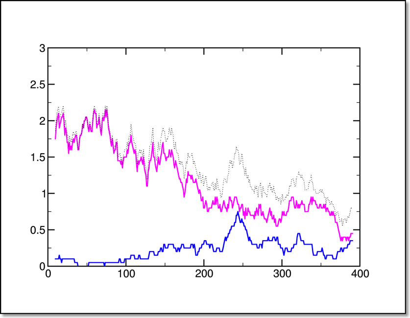
The hydrogen bond data is integer by nature; the best way to present it is averaging over many trajectories of the same type (similar to the way we average the force and work data). Barring that, a quick and dirty way to smooth the data is to use xmgrace to perform a running average (as below). Here we have the latter type in a constant-velocity pulling simulation of the alanine 13-mer.
The lines represent the [i, (i+4)] or alpha (magenta), [i, (i+3)] or 310 (blue) and total (dotted) hydrogen bonds versus time in ps. This same data will be plotted against extension later in this tutorial.
Combining with force/work data
The correspondence between time step and extension is not quite perfect due to the spring-like damping going on in an SMD simulation. Both the force/work data and the hydrogen bond data are arranged according to time step. The trick is to join them appropriately.
The force/work data (a13_smd_all.out) looks like this:
183.20 23.6229 24.1800     2.8684     598.2686
183.30 23.7073 24.1825   -56.3846     598.1276
183.40 23.9375 24.1850   -93.7311     597.8933
183.50 23.5386 24.1875   106.0386     598.1584
183.60 23.3932 24.1900   233.6053     598.7424
183.70 23.1291 24.1925   290.1935     599.4679
The hydrogen bond time series looks like this:
#  Timestep   2       3-10    Alpha     Pi        6        7       total
    0.0       0        0        0        0        0        0        0
    0.1       0        0        0        0        0        0        0
    0.2       0        0        2        0        0        0        2
It is possible to use emacs to join the columns, but anything that requires our manual intervention cannot be automated and therefore takes too long and also gives us the chance to make mistakes. A better alternative is the "join" shell command. In order for the join command to work, the number of data lines must be the same, and the format of the first column must be exactly the same. This is critical. If you examine the data, you will notice that the legend line in the hydrogen bond series needs to be removed (probably we could edit the perl script and have it not output that line to make things easier). Once that is done, and we are sure the number of lines are the same in each file (and the first columns — the x columns — are exactly the same), the command is simple enough:
join a13_smd_all.out a13_smd-hbond-TS.dat > a13_smd_hbond.dat
Drilling down
Now that we have the data all in one place, we can use xmgrace to plot it. We can plot say, the work data and the hbond data against the extension rather than the time step or the actual distance. Because the scales would be very different, we can either use alternate axes, or the overlay method. I think the overlay method is more robust, so we will use it. A brief tutorial on the method is here.
Because the hydrogen bonds are falling, and the work is rising as a function of the extension, this arrangement in this plot makes sense:
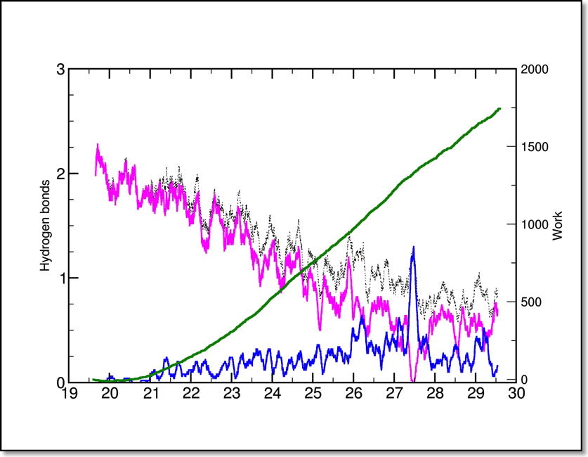
(Notice that the hydrogen bond data looks a bit different than in the time series plot.) In order to accomplish this you should:
- Create a new plot, and read in at least one set of HBond data. You may want to get this data looking how you want it before you proceed.
- Set the axes properly (limits and ticks)
- Create a new overlay. "Edit -> Overlay graphs" then right-click on G0 and "Create new".
- Set "Smart Axis Hints" to "Same X axis scaling"
- Make sure the new (G1) plot in the upper pane is selected, and the old (G0) plot in the lower pane is selected and click "Accept"
You can switch between the two overlays by clicking in the plot area. If you open a "Set Appearance" window, you should notice differences in the data sets when you do this. You will also notice your plot looks a little messed up. You will have to fix these things:
- Read a new data set (work?) into G1. Again, you should be able to use a Set Appearance window to help you figure out which overlay is active. Autoscale only the y-axis when you read it in.
- Sometimes the G1 is smaller than G0. Fix this in the Graph Appearance window under "Viewport -> Xmax".
- Fix the x-axis if it managed to get messed up.