These pages are meant to complement the NAMD Tutorials (here and here) on IMD/SMD. Some of those results will be fleshed out, and some further information on how to obtain results will be given.
Notes on IMD
Web link; NAMD group-provided files for both IMD and SMD are here.
Notes on SMD
Web link of tutorial
Modified files for use with alanine 13-mer may be found here.
This tutorial uses Tcl Forces—it calls a script which has (limited) ability to perform calculations on the fly. This method is different from the one used in the NAMD Tutorial, below. Realize that certain things were done to prepare files for this tutorial which were not mentioned: namely, the vector between the nitrogen atoms on the first and last residue (resid 1:N and resid 10:NT) is defined as the z-axis (in other words, this vector was aligned along the VMD z-axis). Also, the starting PDB has these two atoms 13.7 angstroms apart; during the simulation, these atoms are fixed at 13.0 angstroms apart and moved to 33.0 angstroms apart.
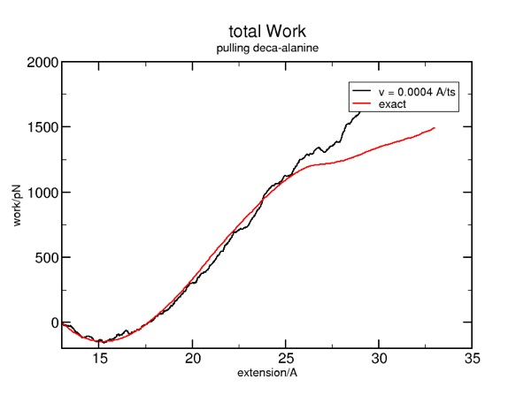
It is natural to want to do two things with this tutorial. First, you may want to improve the quality of the simulation, to see if you can get closer to the exact result for the free energy/work. Second, you may wish to have data files written out, rather than sending the data exclusively to multi plot.
Simulation quality
More is better. But if we simply increase the run time, we will simply stretch the protein to a greater extent. So, what we want to do is increase the run time by say, a factor of five, and also reduce the constant-velocity force by the same factor of five. In the file smd.tcl, find where the velocity is set. By default, it is 0.002. If you reduce it to 0.002/5 or 0.0004, you will need to increase the corresponding run time by the same factor of 5 in order to attain the same extension. Find that in smd.namd: "run 10000 ; 20ps". The new setting would be "run 50000 ; 100 ps".
Notice that the alignment vector is nearly 100% in the z-direction. This is why the forces are adjusted only in the z-direction (smd.tcl):
set f2x [expr ($k*($c2x-$r2x))]
set f2y [expr ($k*($c2y-$r2y))]
set f2z [expr ($k*($c2z+$v*$t-$r2z))]
This is an approximation to the total forces, but a good one.
There is a problem which remains undocumented in the tutorials. Assuming you do everything correctly, the forces that are output by tclForces are MUCH smaller than ones calculated by SMDforce routines (which are examined later). If you look at the two sets, they are the same topologically; there seems to be a simple scaling factor between them. Indeed, I found factor of about 50 through trial and error. After reading separate documentation carefully, the cause is clear: according to this page, the "NAMD unit of force is 1 kcal/mol A ≈ 69.48 pN". Tcl scripting allows you to access the internal NAMD routines directly, so it uses the NAMD unit of force. However, the documentation for SMD forces states the output forces are in pN. This accounts for the mismatch in numbers. The fix is pretty simple. In namd.tcl (or any script you use for tclForces), you scale the NAMD force by 69.48. It is easiest (and safest) to do this at the output stage, so you do not inadvertently apply a too-large force to the atoms (again, in smd.tcl):
set foo [expr $t % $Tclfreq]
if { $foo == 0 } {
set outfile [open $outfilename a]
set time [expr $t*2/1000.0]
# 1 kcal/mol A = 69.48 pN
puts $outfile "$time $r2z [expr $f2z * 69.48]"
close $outfile
Find an appropriately modified smd.tcl file here.
There are two other things you must change in order to properly see the results. The file read.tcl is used to start to display the data with multi plot. Realize that the variables v and dt do not necessarily correspond directly to the pulling velocity and the simulation time step. If you scale the velocity, above, you must scale this velocity variable in read.tcl by the same amount (1/5 = 0.2 in the current case).
Finally, the while loop where the displacement data is strung together must be adjusted slightly, or the number of points won't match.
| while {$i < 33.1} { lappend c $i; set i [expr $i + $v * $dt] } |
| while {$i < 33.0} { lappend c $i; set i [expr $i + $v * $dt] } |
It's probably a good idea to put all these commands into a single tcl script (starting with read.tcl). I've done this with "write_data.tcl", but I remove the multiplot calls — I prefer to plot the data using gnuplot or xmgrace. The initial distance (in the "set i 19.60" line), is the measured distance from VMD between the two TCL atoms. In addition, it's helpful to learn a bit of TCL syntax in order to write to files. This example makes use of internal variable $line. We also use the fact that the end-of-file marker is "-1". What we are really doing is simply reading in the data from our output file, and writing it right back out with some additional data tacked on:
#-- begin file --
set infile [open a13_smd_tcl.out r]
puts "infile"
set outfile [open a13_smd_all.out w]
puts "outfile"
# i should be the true starting distance. This is about 12 for A8,
# about 19.5 for A13 (look at the initial displacement in xxx_smd_tcl.out
# that being said, this is somewhat arbitrary. If the actual distance trails
# the "set" distance, the actual distance can't really be more than the "set"
# at full extenstion. See the last data points for example.
set i 19.60
# v = 1 for original example of v = 0.002 in smd.tcl
# v = 0.25 for 0.0005
# v = 0.05 for 0.0001
# v = 0.025 for 0.00005
set v 0.025
set dt 0.1
set fsum 0
while { [gets $infile line] != -1 } {
set fsum [expr $fsum + [lindex $line 2] * $v * $dt]
puts $outfile "[lindex $line 0] [lindex $line 1] [expr $i + $v * [lindex $line 0]] [lindex $line 2] $fsum "
}
close $infile
close $outfile
# You should plot column 3 as the x
# 2 versus 3 gives actual displacement
# 4 versus 3 gives force
# 4 versus 3 gives work
#
#-- end file --
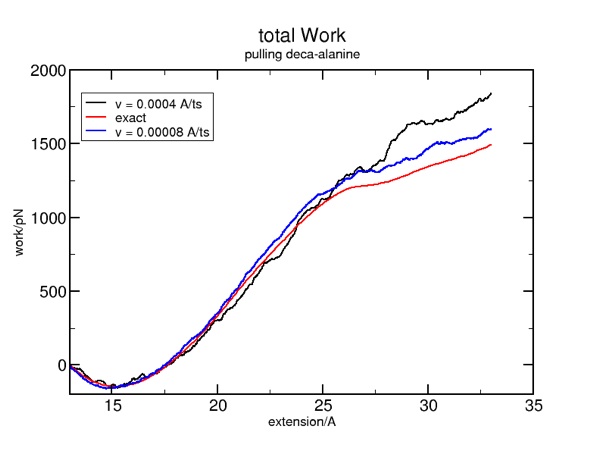
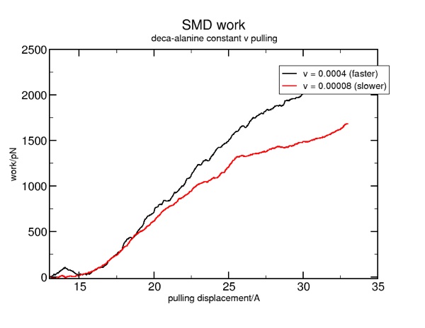
Putting this all together allows you to run some simulations with an even slower pulling velocity, which will get you closer to the exact (reversible) result:
NAMD Tutorial
Web link; Files (tar.gz)
This tutorial is nice to look at as a contrast to the deca-alanine instruction, as it uses a more direct way to calculate the forces. However, it is not as easy to extract the total work/free energy. The setup and running of these simulations is fairly straight forward.
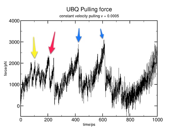
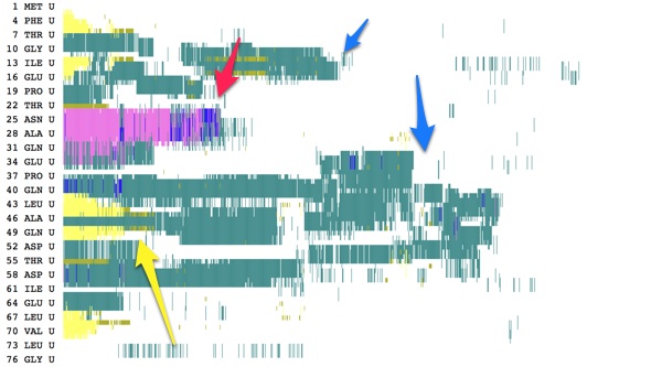
Constant velocity pulling
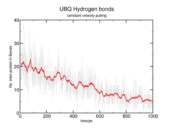
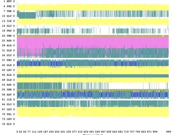
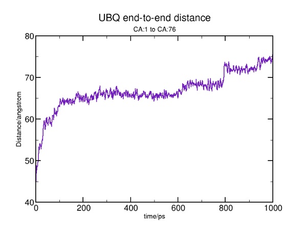
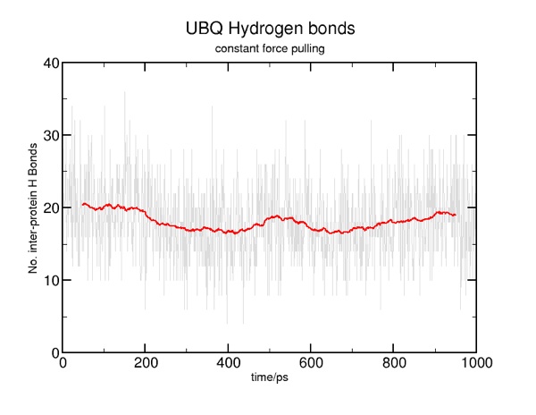
Here are some results from a constant velocity pulling simulation in vacuum. I used SMDk 7, SMDVel 0.0005 and run 500000 (1000 ps/1 ns). You should be able to use the DSS plot along with the hydrogen bond and force data to "see" where structure is breaking. For example, the beta strands lose their cross-linked hydrogen bonds around 100 ps (yellow arrow), and the alpha helix is pulled apart around 200 ps (pink arrow). The other force peaks are where individual coils are fully extended (blue arrows).
Constant force pulling
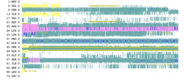
The tutorial has you set a force of 11.5 or so for the moving atom; I found this to be too weak, as you can see from the DSS plot of the trajectory:
Applying a force of 15.0 resulted in some intermediate structures, as seen in the tutorial.
You should carefully consider the difference between constant-force and constant-velocity pulling, and why you might want to use one over the other to investigate certain properties.
Comparing methods: Deca-alanine
In order to see how the two methods arrive at the "same" result, I ran an SMD simulation using the same deca-alanine, fixed atoms, and velocity as in the example, above.
The NAMD configuration file is here. I followed the NAMD tutorial example.
>Main< (SMD_5x) 50 % set allatoms [atomselect top all]
atomselect0
>Main< (SMD_5x) 51 % $allatoms set beta 0
>Main< (SMD_5x) 52 % set fixedatom [atomselect top "resid 1 and name N"]
atomselect1
>Main< (SMD_5x) 53 % $fixedatom set beta 1
>Main< (SMD_5x) 54 % $allatoms set occupancy 0
>Main< (SMD_5x) 55 % set smdatom [atomselect top "resid 10 and name NT"]
atomselect2
>Main< (SMD_5x) 56 % $smdatom set occupancy 1
>Main< (SMD_5x) 57 % $allatoms writepdb da_smd.ref
>Main< (SMD_5x) 58 % set smdpos [lindex [$smdatom get {x y z}] 0]
0.4399999976158142 0.335999995470047 13.40999984741211
>Main< (SMD_5x) 59 % set fixedpos [lindex [$fixedatom get {x y z}] 0]
0.16599999368190765 0.2669999897480011 -0.30399999022483826
>Main< (SMD_5x) 60 % vecnorm [vecsub $smdpos $fixedpos]
0.019975344131504282 0.005030287735711495 0.9997878184055475
>Main< (SMD_5x) 61 %
Notice that the alignment vector is nearly 100% in the z-direction. This is why the TCL scripting example (deca-alanine) looked only at the forces in the z-direction (smd.tcl):
set f2x [expr ($k*($c2x-$r2x))]
set f2y [expr ($k*($c2y-$r2y))]
set f2z [expr ($k*($c2z+$v*$t-$r2z))]
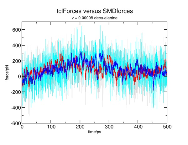
This job runs MUCH faster than the ubiquitin example, so you may wish to run a "10x" version to compare with the corresponding deca-alanine example. Recall the problem with the mis-match in the force units? At this point, they should match in magnitude, as we have applied the fix in smd.tcl. We can check the results of the two methods:
Work and free energy
Once we can be sure that the force units are properly aligned, we may apply the methods used in the tclForces tutorial to the SMD examples. The only difference is the modifying the supplied files to fit the different data.
As you can see, this looks very similar to the tclForces version.