Let's start with the explicitly-solvated 1RNU molecule from Lecture 04. After we are finished, we will compare the dynamics with our implicitly-solvated protein.
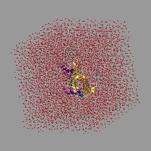
Solvated protein simulation box
Moving on, we need to make sure our simulation box is neutral. This is easy using enerCHARMM.pl:
enerCHARMM.pl -par cmap,blocked -charge 1rnu_TIP3.pdb
1.0000000
In this case, there is a net positive charge, so we need to add a chloride ion:
convpdb.pl -ions CLA:1 1rnu_TIP3.pdb > 1rnu_TIP3_ions.pdb
enerCHARMM.pl -par cmap,blocked -charge 1rnu_TIP3_ions.pdb
0.0000000
(These examples contain many options and switches. Many of them have defaults that work well. A minimal set would be simply
$ minCHARMM.pl -par blocked,cmap -log filename.log INPUT.pdb > OUTPUT.pdb
)
Let's generate a complete PSF of the entire system, and minimize using SHAKE
and PME electrostatics.
genPSF.pl -par cmap,blocked 1rnu_TIP3_ions.pdb > 1rnu_TIP3_ions.psf
minCHARMM.pl -par minsteps=0,sdsteps=500,sdstepsz=0.02 \
-par trunc=switch,cutnb=12,cuton=8,cutoff=11 \
-par blocked,cmap,shake,boxsize=38.743626,nblisttype=bycb \
-cons heavy self 1:13_5 -log mmtsbminsolvate.log \
1rnu_TIP3_ions.pdb > 1rnu_TIP3_ions_min.pdb
Now dynamics in two stages: equilibration ...
mdCHARMM.pl -par cmap,blocked,dynsteps=5000,dynens=NPT \
-par dynitemp=298,dyneqfrq=1000,dynnose=1,dynoutfrq=10 \
-par dynpress=1,echeck=20000,trunc=switch,cutnb=12,cuton=8 \
-par cutoff=11,shake,boxsize=38.743626,nblisttype=bycb \
-log mmtsbdynsolvate.log -enerout 1rnu_cpep_d0.ene \
-trajout 1rnu_cpep_d0.dcd -restout 1rnu_cpep_d0.res \
-final 1rnu_cpep_d0.pdb 1rnu_TIP3_ions_min.pdb
(this took about 30 minutes on my 2.53GHz Intel MacBook Pro)...and production dynamics:
mdCHARMM.pl -par cmap,blocked,dynsteps=5000,dyntemp=298 \
-restart 1rnu_cpep_d0.res \
-par trunc=switch,cutnb=12,cuton=8 \
-par cutoff=11,shake,boxsize=38.743626,nblisttype=bycb \
-log mmtsbdynsolvate1.log -enerout 1rnu_cpep_d1.ene \
-trajout 1rnu_cpep_d1.dcd -restout 1rnu_cpep_d1.res \
-final 1rnu_cpep_d1.pdb 1rnu_cpep_d0.pdb
Specifying a restart file means we don't specify an input PDB.
Analysis---RMSD and RDF
(Although this is VMD-based, you can perform many of these analyses with MMTSB too. Look at the analyzeCHARMM.pl page to investigate further.)
To begin, let's compare the implicit and explicit solvation models against the crystalline structure. Although the two data sets follow approximately the same path, the topology of the data are very different. What similarities and differences can you see in the two models? What do you think it means?
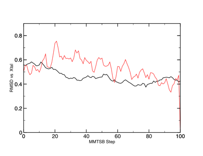
RMSD of 1RNU in implicit (black) and explicit TIP3 (red) solvent.
Next, let's use one of VMD's advanced tools, the Radial Distribution Function calculation tool. Find this under Extensions ➔ Analysis ➔ Radial Pair Distribution Function g(r). An RDF is a histogram of the second selection type (atom) versus distance from the first selection type (atom). For example, if you choose ``OH2'' for both selections, you will get information about the structure of bulk water. Namely, you should be able to see the nearest-neighbor distance, the second-closest neighbor distance, and so on. At large distances, the g(r) should reach the bulk value (which is usually normalized to 1, no matter the actual pairs involved).
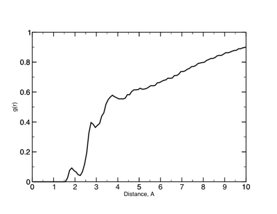
g(r) between the protein (surface) atoms and water oxygens.
Thus, this tool requires two selections, which are usually atom names. The other thing to be sure to set is the maximum r (distance); this should be no more than 1/2 the box size (you should also understand why; to find out, read up on periodic boundary conditions). Once you have the settings right (don't forget to specify a file to save data to), hit ``Compute g(r)'', and see how it looks. RDFs are used very commonly in simulation studies to check on contacts and local structure, as well as sanity checks on things like bulk behavior.
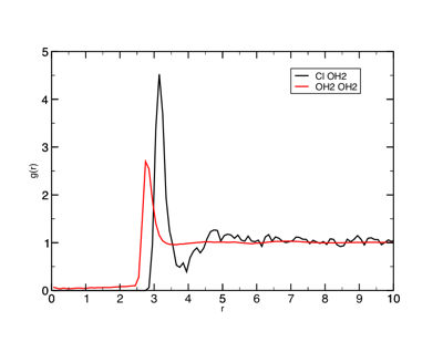
g(r) between the chloride ions and water oxygens.
The fewer the number of atoms you are counting, the noisier the data. For example, compare the Cl— -- OH2 RDF in the above Figure with the OH2 OH2 RDF (the scales are the same). What do you think the height of the peak tells you about the structure?
Analysis---Ramachandran Plots
Another interesting analysis tool is the Ramachandran Plot tool. This plots the familiar Ramachandran plot in Ψ,φ space (you have to make sure to select your molecule; by default, no molecule is selected!). It will even show it dynamically as your trajectory runs. It has common secondary (Ψ,φ)-space areas marked on the plot. In addition, it will create a 3D histogram of the data (as a new molecule object in the main VMD window). You will probably wish to generate data in MMTSB for a nicer-looking 3D plot, however (Ramaplot will not save the dataset to a file for you). In order to use this, you will have to render the window to an image file.
So how to get a more conventional Ramachandran plot? You can either use the Timeline, and write out both the Ψ and φ values, then combine those files. Assuming your data is called phi.dat and psi.dat, you may use some of the scripting we tried earlier in the course (called makePsiPhi.csh for this purpose):
#!/bin/csh
grep 'P CA' phi.dat | cut -c1-28 > phi1.tmp
grep 'P CA' psi.dat | cut -c1-28 > psi1.tmp
paste phi1.tmp psi1.tmp > PhiPsi.tmp
grep -v '0.0' PhiPsi.tmp > PhiPsi.dat
rm -rf *.tmp
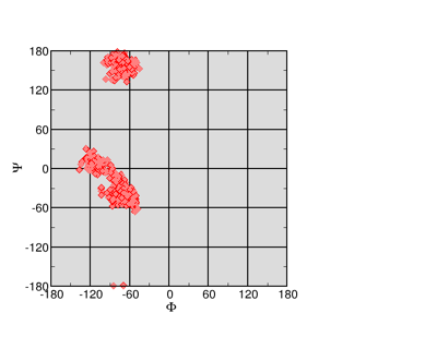
Ramachandran Plot
Note that this culls some of the data---residues at the end of our 1RNU protein are not helical. Thus there is a lot of zeroes in our data. On the left is the result (using Xmgrace). Ramachandran plots are useful, but if you include large sections of the protein you will probably show more than you intended. It is best to filter your data (or limit your selection in VMD) in order to show only the parts of the protein that you are directly focused on.
Analysis—Hydrogen Bonding
Counting the number of hydrogen bonds is in principle easy to do. In the old days, this required a separate call to a CHARMM hydrogen-bond counting routine along with defining different donors and acceptors. Now, VMD allows hydrogen bonds to be counted easily. The Timeline tool provides a graphical solution, but the best solution is probably the Extensions ➔ Analysis ➔ Hydrogen Bond tool. (Side note: CHARMM and VMD probably calculate exactly what constitutes a hydrogen bond somewhat differently. There are in fact, many different ways to define a hydrogen bond, based upon angles, distances, residue inclusion, and so on.)
The tool requires at least one selection---for example, protein. In the case of 1RNU, the number of hydrogen bonds will be counted within the protein/helix. In addition, the parameters such as Hbond distance and angle may be specified. As usual, a plot is put up, and data may be written to a file. The data is very granular, as of course only integer number of hydrogen bonds may exist per step.
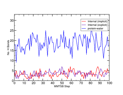
Time-dependent hydrogen bonds in the 1RNU simulations. Note that the implicit simulation produces zero protein-water hydrogen bonds.
For an implicitly-solvated system, the only hydrogen bonds will be within the protein. For an TIP3-solvated system, however, hydrogen bonds will also be formed with the water molecules. It may be interesting to consider not only whether the GB and TIP3 solvation models give similar in-protein hydrogen bonds, but how many hydrogen bonds the TIP3 solvent provides to the protein (in which case, one may be able to count how many water molecules lie in a bound, first solvation shell).