Assuming that you have found a protein (or smaller molecule or fragment) at www.rcsb.org that you would like to study with MD, you must of course prepare what you are given for CHARMM. Here is how we do it.
First steps: download
If you visit the protein databank, there are many options. Somewhere on the page, you will find a Download Files link (as of August, 2013, it is near the upper-righthand corner). For simplicity's sake, let's simply download the PDB file, and save it somewhere convenient.
You do have to know a bit about the PDB file. It may consist of separate "chains"— substituent parts of the protein which may or may not be similar to each other. Usually, you can determine this information with careful reading of the header/comments in the top of the PDB file. For example, here is the beginning of the header of 1RNU:
HEADER HYDROLASE(PHOSPHORIC DIESTER,RNA) 19-FEB-92 1RNU
TITLE REFINEMENT OF THE CRYSTAL STRUCTURE OF RIBONUCLEASE S.
TITLE 2 COMPARISON WITH AND BETWEEN THE VARIOUS RIBONUCLEASE A
TITLE 3 STRUCTURES
COMPND MOL_ID: 1;
COMPND 2 MOLECULE: RIBONUCLEASE S;
COMPND 3 CHAIN: A;
From this we can see there is only one chain, chain A. The header continues on and gives all kinds of useful information:
SEQRES 1 A 124 LYS GLU THR ALA ALA ALA LYS PHE GLU ARG GLN HIS MET
SEQRES 2 A 124 ASP SER SER THR SER ALA ALA SER SER SER ASN TYR CYS
SEQRES 3 A 124 ASN GLN MET MET LYS SER ARG ASN LEU THR LYS ASP ARG
SEQRES 4 A 124 CYS LYS PRO VAL ASN THR PHE VAL HIS GLU SER LEU ALA
SEQRES 5 A 124 ASP VAL GLN ALA VAL CYS SER GLN LYS ASN VAL ALA CYS
SEQRES 6 A 124 LYS ASN GLY GLN THR ASN CYS TYR GLN SER TYR SER THR
SEQRES 7 A 124 MET SER ILE THR ASP CYS ARG GLU THR GLY SER SER LYS
SEQRES 8 A 124 TYR PRO ASN CYS ALA TYR LYS THR THR GLN ALA ASN LYS
SEQRES 9 A 124 HIS ILE ILE VAL ALA CYS GLU GLY ASN PRO TYR VAL PRO
SEQRES 10 A 124 VAL HIS PHE ASP ALA SER VAL
HET SO4 A 125 5
HETNAM SO4 SULFATE ION
FORMUL 2 SO4 O4 S 2-
FORMUL 3 HOH *88(H2 O)
HELIX 1 H1 THR A 3 MET A 13 1 11
HELIX 2 H2 ASN A 24 ASN A 34 134 IN 310 CONFORMATION 11
HELIX 3 H3 SER A 50 GLN A 60 156 - 60 IN 310 CONFORMATION 11
SHEET 1 S1 3 LYS A 41 HIS A 48 0
SHEET 2 S1 3 MET A 79 THR A 87 -1
SHEET 3 S1 3 ALA A 96 LYS A 104 -1
SHEET 1 S2 4 LYS A 61 ALA A 64 0
SHEET 2 S2 4 ASN A 71 SER A 75 -1
SHEET 3 S2 4 HIS A 105 GLU A 111 -1
SHEET 4 S2 4 VAL A 116 VAL A 124 -1
SSBOND 1 CYS A 26 CYS A 84 1555 1555 2.01
SSBOND 2 CYS A 40 CYS A 95 1555 1555 2.01
SSBOND 3 CYS A 58 CYS A 110 1555 1555 2.01
SSBOND 4 CYS A 65 CYS A 72 1555 1555 2.02
CISPEP 1 TYR A 92 PRO A 93 0 7.32
CISPEP 2 ASN A 113 PRO A 114 0 -0.39
SITE 1 ACT 9 HIS A 12 LYS A 41 VAL A 43 ASN A 44
SITE 2 ACT 9 THR A 45 HIS A 119 PHE A 120 ASP A 121
Another way to determine chain information is to look at the coordinates, and find the "chain" column, which occurs after the residue/peptide label (see above).
One thing to realize in preparing simulation files is that simulation software generally wants to group according to different molecules or molecule types. PDB files acquired from the RCSB do not distinguish between these, generally. For example, our 1RNU.pdb structure contains the protein, a sulfate, and many water (HOH) molecules. The crystallographic waters ARE included as part of the single chain (Chain A), so these need to be removed.
You can often remove these things by using the "-nohetero'' switch. This should also remove "funny" residues that may not exist or are not peptides: SO4, AMP, etc. This switch depends upon the HETATM label being present on these residues. The original 1RNU.pdb (obtained from the RSCB) is configured this way. However, convpdb.pl will change those HETATM notations to ATOM in the PDB file! This means we need to strip out those atoms FIRST. See what happens if I run another convpdb.pl command:
Original 1RNU.pdb:
ATOM 949 CB VAL A 124 -6.191 -19.227 3.293 1.00 39.17 C
ATOM 950 CG1 VAL A 124 -5.637 -20.488 2.672 1.00 45.64 C
ATOM 951 CG2 VAL A 124 -5.194 -18.092 3.116 1.00 37.17 C
ATOM 952 OXT VAL A 124 -8.956 -20.594 1.649 1.00 56.65 O
TER 953 VAL A 124
HETATM 954 S SO4 A 125 -9.453 -3.716 7.958 1.00 31.29 S
HETATM 955 O1 SO4 A 125 -10.444 -3.588 6.961 1.00 48.25 O
HETATM 956 O2 SO4 A 125 -9.360 -2.524 8.744 1.00 67.13 O
HETATM 957 O3 SO4 A 125 -8.179 -3.989 7.418 1.00 71.29 O
HETATM 958 O4 SO4 A 125 -9.837 -4.775 8.813 1.00 37.89 O
HETATM 959 O HOH A 126 -7.113 -3.457 20.325 1.00 23.42 O
HETATM 960 O HOH A 127 -18.875 1.354 16.321 1.00 25.11 O
(Notice that only the oxygen atoms of the waters "HOH" are reported.)
1RNU output after 'convpdb.pl -chain A':
ATOM 949 CB VAL A 124 -6.191 -19.227 3.293 1.00 39.17
ATOM 950 CG1 VAL A 124 -5.637 -20.488 2.672 1.00 45.64
ATOM 951 CG2 VAL A 124 -5.194 -18.092 3.116 1.00 37.17
ATOM 952 OXT VAL A 124 -8.956 -20.594 1.649 1.00 56.65
ATOM 954 S SO4 A 125 -9.453 -3.716 7.958 1.00 31.29
ATOM 955 O1 SO4 A 125 -10.444 -3.588 6.961 1.00 48.25
ATOM 956 O2 SO4 A 125 -9.360 -2.524 8.744 1.00 67.13
ATOM 957 O3 SO4 A 125 -8.179 -3.989 7.418 1.00 71.29
ATOM 958 O4 SO4 A 125 -9.837 -4.775 8.813 1.00 37.89
ATOM 959 O TIP3A 126 -7.113 -3.457 20.325 1.00 23.42
ATOM 960 O TIP3A 127 -18.875 1.354 16.321 1.00 25.11
(Notice that convpdb.pl has CHANGED not only HETATM -> ATOM but HOH -> TIP3! This is a feature, but it is inconvenient if you don't know it is happening!)
You will not extract "extra" residues from such a modified (by convpdb.pl) PDB file if you throw the '-nohetero' switch (try it!). We can fix this, however. In this case, we need to use the '-exclude' switch, along with the residue numbers of the residues to remove. You must examine your PDB file to find out which these are. In the case of 1RNU, we see the spot where the protein ends, and the "other" residues (sulfate and water) show up. The first non-protein residue is 125, and the last (look at the last lines) is 213. So issuing this command:
convpdb.pl -exclude 125:213 1RNU.pdb > 1RNU-protein.pdb
Will remove all those spurious residues.
IF the file does contain separate chains, you should also extract each into its own PDB file. You can do this with the -chain switch:
$ convpdb.pl -chain A PROTEIN.pdb > PROTEIN_A.pdb
$ convpdb.pl -chain B PROTEIN.pdb > PROTEIN_B.pdb
..and so on. Our particular example (1RNU) only has ONE chain, so you need not do this step for 1RNU.
Lastly, because you have taken out some residues, the numbering will not be contiguous. This will present a problem for simulation software at various stages. We can renumber the residues (from "1" or any number). See for example this tutorial.
$ convpdb.pl -renumber 1 PROTEIN_A.pdb > PROTEIN_A_renum.pdb
If the protein has been mutated, you may wish to set it back to its natural state. Or, you may wish to mutate it! This is easy using mutate.pl. Let's mutate our protein. Find a residue (say a cysteine) and mutate it to say serine. (According to the MMTSB documentation,mutate.pl does not like chain IDs, so you must set the chain ID to an empty character first, then set it back to what it was before.)
convpdb.pl -setchain " " PROTEIN_A_renum.pdb | mutate.pl -seq 110:S | \
convpdb.pl -setchain A > PROTEIN_A.mutated.pdb
(To do this, we didn't really need to know that residue 110 was a CYS—but you probably should know what type of residue you are mutating!)
Once you have done these things, you can see if CHARMM will minimize the structure. This is a quick and dirty way to find out if you are on the right track. Remember that minimization is also an easy way to add missing hydrogens to your structure (convpdb.pl can also run a minimization; see the manual page).
1RNU example--Keeping crystal waters
We can put all this together in the context of our 1RNU molecule. First, extract just the protein part, and renumber the residues:
convpdb.pl -nohetero -renumber 1 1RNU.pdb > 1RNU-protein.pdb
Next, extract the existing water molecules (from the original PDB). This is done in three steps: selection/extraction (renumbering from 1), and adding hydrogens (to the oxygen atoms remembering that the original PDB only contained the positions of the oxygen atoms):
convpdb.pl -nsel water -renumber 1 1RNU.pdb |complete.pl > 1RNU-tmp.pdb
(here, I was able to string two commands together with a "pipe" — the "|" character. Output from the first step is fed directly to the second command.) Next, we write out the result with an appropriate chain label:
convpdb.pl -setchain X 1RNU-tmp.pdb > 1RNU-xraywater.pdb
Finally, we will recombine these waters with the stripped-down structure:
convpdb.pl -merge 1RNU-xraywater.pdb 1RNU-protein.pdb \
> 1RNU-complexwaters.pdb
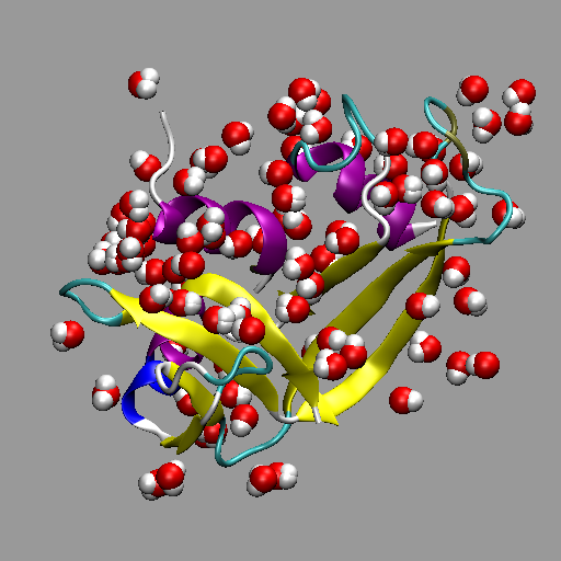
Crystallographic waters contained within an RCSB PDB.
Now we can perform the full solvation. Later on, we will do this in more detail. For now, we may issue this command, which creates a cubic box and keeps at least 9 angstroms between any new waters and the protein and its crystal waters. NOTE: August, 2013. The 'convpdb.pl -solvate' command is broken for some reason. In this case, you need to solvate the structure in VMD, as we learned how to do earlier in the semester. This probably means sending your PDB file back to your PC/Mac so you can use VMD to solvate it. Then, you must send the resulting fully-solvated structure back to the remote machine so you may run VMD. OR you may may simply run the solvated structure through NAMD on your PC/Mac!
convpdb.pl -solvate -cutoff 8 -cubic 1RNU-complexwaters.pdb \
> 1RNU-solvated.pdb
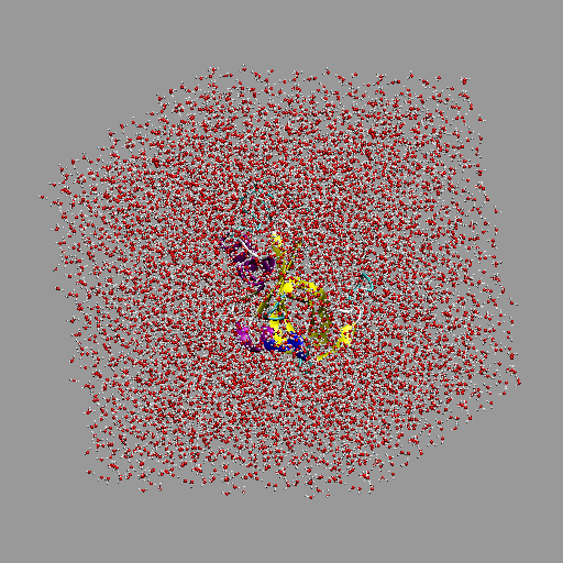
Solvated 1RNU protein simulation box.
Implicit Solvation models
Now that we know how to create a protein in a box of water, let's take a step back, and talk about solvation in general. While explicit solvation generally gives more realistic results, it is much more computationally intensive than implicit models. Implicit models treat solvent as a continuum, with either constant or varying dielectric constant ε (epsilon). The most commonly-used such model is the Generalized Born model of solvation (GB or GBMV).
The protein should still be minimized. We can prepare for our GB simulation thus:
minCHARMM.pl -par blocked,cmap 1RNU-protein.pdb > 1RNU-protein-min.pdb
Starting with a bare protein PDB, we can easily invoke the Generalized Born method by using the '-par gb' switch (there are often other things added to this). In the following, we also illustrate an alternative way to accomplish heating (three separate steps). Note that the last PDB listed is the INPUT file, and the argument to the "-final" switch is the OUTPUT file. The output file from each step becomes the input file for the next step.
mdCHARMM.pl -par gb,blocked,cmap,dynsteps=5000,dyntemp=100 \
-final 1rnu_GB_100.pdb 1RNU-protein-min.pdb
mdCHARMM.pl -par gb,blocked,cmap,dynsteps=5000,dyntemp=200 \
-final 1rnu_GB_200.pdb 1rnu_GB_100.pdb
mdCHARMM.pl -par gb,blocked,cmap,dynsteps=5000,dyntemp=300 \
-final 1rnu_GB_300.pdb 1rnu_GB_200.pdb
The GB method treats the solvent-solute potential energy interactions, but does not account for any "bouncing'' or friction between the molecules. In order to simulate this effect, we turn on Langevin dynamics with a friction term (langfbeta=10):
mdCHARMM.pl -par blocked,cmap,gb,dynsteps=5000 \
-par dyntemp=300,dynoutfrq=10,lang,langfbeta=10 \
-trajout 1rnu_gb_300_prod.dcd \
-final 1rnu_GB_300_PROD.pdb 1rnu_GB_300.pdb
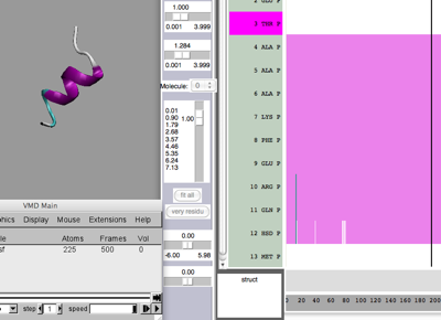
Secondary Structure/Timeline
Now that we have some data, let's do some analysis. Load the DCD into the PSF file in VMD. Assuming that you understand how to perform RMSD trajectory analyses, let's move on to something else. Open up the Timeline tool ( Extensions ➔ Analysis ➔ Timeline). The Timeline tool allows you to examine your structure through its sequence. Very roughly, it will plot time-based data against the sequence. To see this, select "Calc. Sec. Struct.'' under the Calculate menu. After cycling through all the trajectory frames, it will give a color-based representation of the secondary structure (pink is an α-helix, blue is a 310 helix, yellow is a β-sheet, etc.).
You may select a secondary-structure based representation in VMD to match what you see in the timeline dynamically. Under the Main VMD menu, choose "Graphics ➔ Representations'". Under the Graphical Representations menu that pops up, choose Coloring method ➔ Secondary Structure and Drawing Method ➔ New Cartoon. You should run the trajectory and see how the timeline matches up to the view.
One thing to realize is that this VMD view is not updated frame-by-frame. In other words, the secondary structure of whatever frame you happen to be on is chosen to represent every frame To see this, find a frame in your Timeline which is not an alpha-helix. You can click above the time scale and a vertical line will appear, and the trajectory will be moved to that frame. Key on the frame you want to select, and re-draw the secondary structure representation.
In order to make each frame accurately reflect the secondary structure, we need to use a script which will check each frame. The script is called sscache (find it here). (Put it somewhere; my suggestion is ~/vmd/scripts/tcl.) Once you have downloaded it, you need to run it from a VMD terminal (Extensions ➔ Tk Console) Assuming your molecule of interest is number 0, you invoke it thus:
$ source ~/vmd/scripts/tcl/sscache.tcl
$ start_sscache 0
Now, re-run your trajectory, and you should notice some changes in the representation and color of your molecule.
Timeline
(movie without and with sschche??)
When you clicked on your Timeline, you may have noticed you created a new selection and representation of your molecule. For large proteins, this is a convenient way to select contiguous regions. The default representation is "Bonds'', but this can be changed easily after selection.
Other Timeline analyses
There are other analyses available such as $\psi$-$\phi$ angles; Let's look at hydrogen bonds. If you select Calc. H-Bonds under Calculate, you will now see a list of hydrogen bond triplets (the O-H-N atoms). But you probably won't see any features. Go to Threshold and set the lower bound to 0, and the upper bound to above 1, but below 2. Once set, you should see a plot of active (light) and inactive (dark) hydrogen bonds.
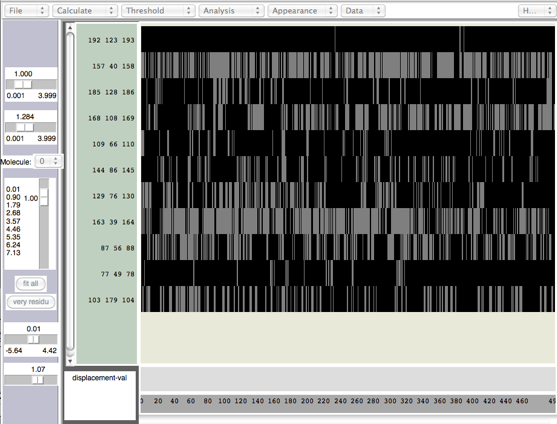
Hydrogen bonds in Timeline
Another way to find hydrogen bonds is with the Extensions ➔ Analysis ➔ Hydrogen Bonds tool. Open this tool up and have a look. It may be useful to export the file so you can plot it in your favorite plotting program (more on this later on in the course).
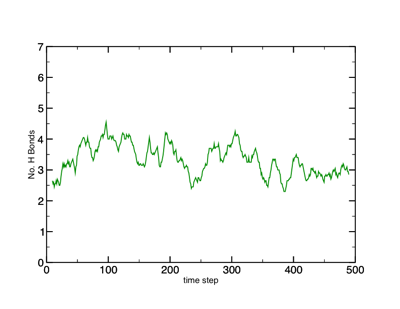
Hydrogen bond plot.