Steered Molecular Dynamics or SMD
(Click here for the files)
Motivation
In steered molecular dynamics (SMD), an outside force is applied to one or more atoms in a molecule, and usually, another part of the molecule is "nailed down" so that the outside force(s) do not merely move the whole molecule through space. For peptides, proteins , DNA and/or RNA, this can stretch or break different secondary-structural features, beginning with hydrogen bonds (as they are the weakest and most prevalent forces determining secondary structure), but also including other non-covalent forces such as dipole-dipole or ionic attractions. Many physical insights can be observed from such artificially-manipulated systems. The perturbations may be applied as constant-force, or constant-velocity. Take some time to think about how these differ, and what might be the advantages and/or disadvantages of each method.
As one example, consider the simple pulling of a polyalanine. A naive model of such a helical peptide is a coiled wall phone cord. As a phone cord is stretched, the coils become more tightly wound, and the stretching is accomplished while maintaining the coil. This is at least party because of the way the phone cord is physically held (the ends may not rotate unless you create such a clamping mechanism). In a helical peptide, this is not quite the case. While there is some narrowing of the diameter of the helical barrel, there is also an unwinding due to the fact that 1) the ends of the peptide (indeed, all the backbone bonds) may rotate freely, and 2) the coiling of the peptide is held by granular hydrogen bonds, not the material itself.
This second example is similar, but this time a sodium ion is placed at the C-terminal end of a helical peptide, which is then pulled. The peptide is non-covalently bonded to the sodium ion, and it pulls along with it, unwinding the helix from the fixed end. The alpha helical parts of the protein are dynamically rendered as a purple ribbon, and 3-10 helix as blue. Notice the rotation, and how the C-terminal carbonyl oxygens claw the sodium ion.
As another example, we can stretch a monomer unit of titan, which provides the elasticity in muscles. In this movie, the secondary structure is continually updated, and the hydrogen bonds present are also indicated in each frame.
SMD: Lu, etal, Biophysical Journal 75, 662 — 671 (1998) and AFM experiments: Rief, etal, Science 276, 1109 — 1112 (1997)
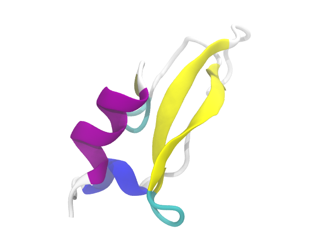
For our example of SMD, we will utilize the familiar 1QLQ molecule. This has some nice features which make it attractive for SMD: well-defined and small secondary-structural regions (3-10 helix, alpha helix, and beta sheets), and the ends are easy to pick out and use for the fixed and pulled ends.
Preparation and Background
The steps involved for an SMD simulation are
- Create a matched PSF/PDB pair, using the methods we have learned so far
- Identifying likely anchor (fixed atom(s)) candidates and pulled atom(s)
- Using VMD to collect labeling information on these atoms (resname, name, index, etc)
- Determining the type of SMD simulation — Constant force or constant velocity
- Inserting the necessary lines into a NAMD control file which will identify the simulation as an SMD simulation
- Creating/editing a TCL file that specifies necessary parameters
- Running a test simulation, processing the results, and fine tuning any of the above
- Creating multiple copies of the simulation, and running them in sequence
- Processing the individual results, and combining the data into one "averaged" result
(The items in red are things we need to learn here!)
In our example, we will use a constant velocity SMD simulation. The differences and effects are discussed in a lecture video.
As in most other simulations, we are going to start off the by equilibrating our molecule. This time, with a view towards running a number of independent simulations and combining the resulting data, we are going to do extract a number of coordinate sets from an equilibrated trajectory (DCD file) by saving the coordinates in VMD.
If you choose an SMD simulation for your final project, part of the assignment will require multiple simulation runs to average. In other words, we will repeat the experiment for better statistics. You could run five separate simulations, waiting for each on to finish before starting the next one. But it is much more efficient to automate this process by using a terminal or shell script. Before we do that, however, we want to run a single equilibration simulation, from which we will take 5-10 sets of coordinates (write out PDB files) to use as starting points for the different SMD experiments.
Now let's look at the files included for this laboratory (link above):
- 1qlq_solvated.pdb, 1qlq_solvated.psf – the PSF/PDB pair (includes water molecules, this is OK!)
- 1qlq_fixed.pdb, 1qlq_fixed.psf – a PS/PDB pair which specifies which atoms are fixed. THESE ARE NOT USED IN THIS LABORATORY, but are provided in case you want to start a simulation totally from scratch.
- 1qlq_SMD.conf – the NAMD control file
- Equilibration.conf – the NAMD control file to run an equilibration of 1QLQ
- smd.tcl – TCL script which specifies fixed and pulled atoms, and force/velocity settings
- write_data.tcl – TCL script which uses NAMD output to extract force/distance data
- multi.csh – csh script which combines multiple simulation data into an averaged set
- par_all22_prot_cmap.inp – the parameter file that was used to generate the PSF and PDB.
You should now be able to put these all together to produce some output, in particular the output 1qlq_smd_tcl.out, which will contain our force data. To get there, you should be able to run all the supplied files without modification. We will do that, and then explain the specifics needed to change this for other molecules.
Running the Equilibration Simulation
First, run the equilibration simulation:
namd2 +p4 Equilibration.conf > Equilibration.log
Next, let's extract a single frame from the equilibrated system to use for our SMD simulation. Load the PSF and DCD into VMD, and save one frame as a PDB file called "1qlq_EQ.pdb". If you are not sure how to do this, review the laboratories in Weeks 2 and 3.
Loading the equilibrated system (In a VMD tkcon):
mol load psf 1qlq_solvated.psf dcd 1qlq_solvated_eq.dcd
There are ways to write TCL script for the tkcon which will automate the writing of separate files. For now, let's approximate that process. Here are some useful tkcon commands:
(IN A tkcon)
animate goto xxx
This advances the dcd to frame xxx
animate write pdb 1qlq_EQ.pdb
This will write a PDB of the current frame to the file 1qlq_EQ.pdb. You can use relative or absolute paths to put this file anywhere. For example
animate write pdb run1/1qlq_EQ.pdb
will write the PDB to the directory "run1" below the current directory.
Using these commands will allow you to write independent PDB files to separate run-time directories.
Running the SMD Simulation
Once you save a single PDB as 1qlq_EQ.pdb, you should be able to run the actual SMD simulation:
(in a terminal):
namd2 +p4 1qlq_SMD.conf > 1qlq_SMD.log
(This will take some time on your computer, perhaps 30 minutes or more.)
At this point, you should load these results into VMD and make sure you see evidence of pulling. Hint: because all these simulations share the same PSF, you do not have to create new molecules. You may delete frames from your previously loaded equilibration simulation, and load in the SMD simulation DCD file(s). What evidence do you see?
Now that we can see what happens, let's see how it works. First, the part of the control file (1qlq_SMD.conf) that is different from what we have seen before are these lines:
# Tcl interface
tclForces on
tclForcesScript smd.tcl
This tells NAMD that outside forces will be used, and the details are in the file smd.tcl. Let's look at smd.tcl and pick out the important parts, annotated in red. These annotations are NOT in the original file. They are added here to help explain what things you would have to adjust for your own simulation. Most of this file (in grey) would not need to be changed if you chose a different molecule to work with.
# $Id: smd.tcl,v 1.2 2005/02/18 18:07:11 mbach Exp $
# Atoms selected for force application
# "BH" is molecule name (probably "PEP" or "PRO0")
set id1 [atomid MAIN 1 CA] <—— This is the PULLED atom information
set grp1 {}
lappend grp1 $id1
set a1 [addgroup $grp1]
set id2 [atomid MAIN 58 CA] <--- This is the FIXED atom information
set grp2 {}
lappend grp2 $id2
set a2 [addgroup $grp2]
# set the output frequency, initialize the time counter
set Tclfreq 50
set t 0
# constraint points
# these should closely match actual positions.
# a13 gives a distance via VMD of 19.61
set c1x 39.872 <—
set c1y 20.811 <—— Here are the initial PULLED atom coordinates, taken from the initial structure.
set c1z 8.488 <—
set c2x 42.060 <—
set c2y 24.023 <—— Here are the initial FIXED atom coordinates, taken from the initial structure.
set c2z 4.656 <—
# force constant (kcal/mol/A^2)
set k 7.2
# pulling velocity (A/timestep)
set v 0.005 <— Here is the (constant) velocity in A/timestep. Everything after this point will not need to be changed.
set outfilename 1qlq_smd_tcl.out
open $outfilename w
proc calcforces {} {
global Tclfreq t k v a1 a2 c1x c1y c1z c2x c2y c2z outfilename
# get coordinates
loadcoords coordinate
set r1 $coordinate($a1)
set r1x [lindex $r1 0]
set r1y [lindex $r1 1]
set r1z [lindex $r1 2]
set r2 $coordinate($a2)
set r2x [lindex $r2 0]
set r2y [lindex $r2 1]
set r2z [lindex $r2 2]
# calculate forces
set f1x [expr $k*($c1x-$r1x)]
set f1y [expr $k*($c1y-$r1y)]
set f1z [expr $k*($c1z-$r1z)]
lappend f1 $f1x $f1y $f1z
set f2x [expr $k*($c2x-$r2x)]
set f2y [expr $k*($c2y-$r2y)]
set f2z [expr $k*($c2z+$v*$t-$r2z)]
lappend f2 $f2x $f2y $f2z
# apply forces
addforce $a1 $f1
addforce $a2 $f2
# output
set foo [expr $t % $Tclfreq]
if { $foo == 0 } {
set outfile [open $outfilename a]
set time [expr $t*2/1000.0]
# MODIFIED to provide units in pN
# 1 kcal/mol A = 69.48 pN
# also because r1z is not 0.0, need to find true distance
puts $outfile "$time [expr $r2z - $r1z] [expr $f2z * 69.48]"
# puts $outfile "$time $r2z $f2z"
close $outfile
}
incr t
return
}
Some things have been simplified here. Most importantly, the direction of pulling relative to the molecule has not been well-defined. In general when working with a new molecule, you must:
- Align the molecule/system in a particular coordinate direction (say along the z-axis). This is typically done with the orient plugin in VMD.
- Specify the orientation of the pulling.
Now, let's turn to the results. The data is written to a file called 1qlq_smd_tcl.out. Here are the first six lines:
(time in ns, displacement, force)
0.0 -3.4940140630310648 183.1053680777846
0.1 -3.535559294397924 315.5346513133925
0.2 -3.5334575685641205 414.14082385833416
0.3 -3.5421488819547067 531.7797122615509
0.4 -3.5277758715508503 622.9702775479278
0.5 -3.522895839531471 727.4149583144
Remember that the carbon end is pulled indirectly. This means first of all that the initial displacements are very random, even negative, and noisy. Think of this as analogous to the heating phase of a conventional simulation. It is also important to decide what your dependent variable (x-axis) should be: time (really tilmestep) or displacement. Whichever you decide, you should present all your data in terms of this variable. This may require some data manipulation! In the following figures, tilmestep is used for simplicity.
Nuts and Bolts Example
See also the SMD Video lectures, parts 1 and 2.
Below is an example of a script that can be used to run multiple different SMD simulations, use it as your guide. Once it is edited to your liking, run it in terminal by entering the script name then the number of runs. This is saved to a file, (for example 5runs.csh), and the file would have to be made executable with
chmod 755 5runs.csh
An explicit example of a simpler C-shell script was given in a lecture video. You could combine the lecture example with this script to create each directory before namd2 is called.
#!/bin/csh
set nrun = $1
set suff = 1
while ( $suff <= $nrun )
cd Run_$suff
namd2 +p2 1qlq_SMD.namd > 1qlq_SMD.log
cd ..
@ suff++
end
As an explanation,
- #!/bin/csh – this "hash bang" identifies the type of shell language that will run this script (the C Shell or csh)
- set run = $1 – this says that a variable (nrun) will be set to the argument passed when we run the script file.
- set stuff = 1 – this says that a new variable "suff" is created and it's value is set to 1.
- while (. . .) – this starts a loop, which will continue as long as the value of suff is less than or equal to nrun.
- (in the loop) cd Run_$suff – change to the directory Run_1 (first time through the loop)
- (in the loop) namd2 +p2 1qlq_SMD.namd > 1qlq_SMD.log – run NAMD using the config file 1qlq_SMD.namd, and send the output to 1qlq_SMD.log
- (in the loop) /usr/bin/tclsh write_data.tcl – process the output to get the force data (uses the file write_data.tcl to do this)
- (in the loop) cp 1qlq_smd_frames.coor . . . – copy (processed) coordinates to a PDB file
- (in the loop) cd .. – move out of this run directory
- (in the loop) @ suff ++ – increment the value of suff by +1
- end – this returns us to the top of the loop
This script file would be run by simply calling it with one argument (the number of runs you wish to perform):
5runs.csh 10
One of the tough things about programming (we call this scripting, but it is a form of programming!), is variables. In scripting, when you set a variable, you use the plain variable name. When you REFER to a variable, you have to use the variable signal "$" in front of it. This is especially confusing when looking at the first occurrence:
set nrun = $1
Here, we are setting the variable nrun to a value, so we do NOT say "$nrun". But, that value is the value of a variable which has already been set, 1 (which, by the way, is a system or default variable representing the first argument of a command passed to a program; $2 would refer to the second argument, and so on), which must be represented by $1. Confusing!
Examples of individual versus averaged data
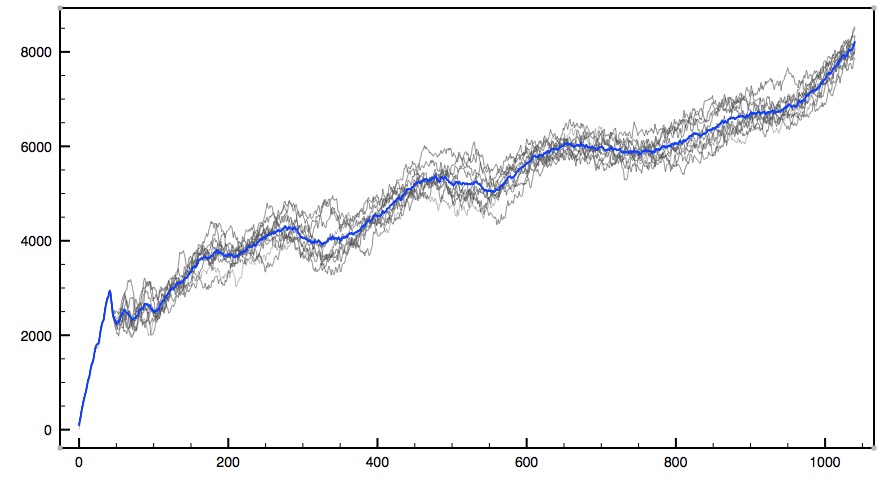
This plot is force (in pN/A) versus simulation time step. A plot of force versus displacement should be similar, and each individual run result should look more or less like one grey line. Each drop or dip signifies an important hydrogen bond breaking. The blue line is an average of the ten simulations. Even though variations between individual simulations appear quite large, upon averaging, certain patterns do present themselves.
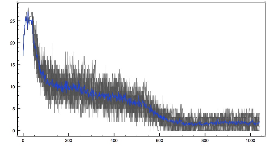
This plot shows the number of hydrogen bonds versus time step. Data for 10 individual simulations (grey) are superimposed. The blue line is an average of these data.
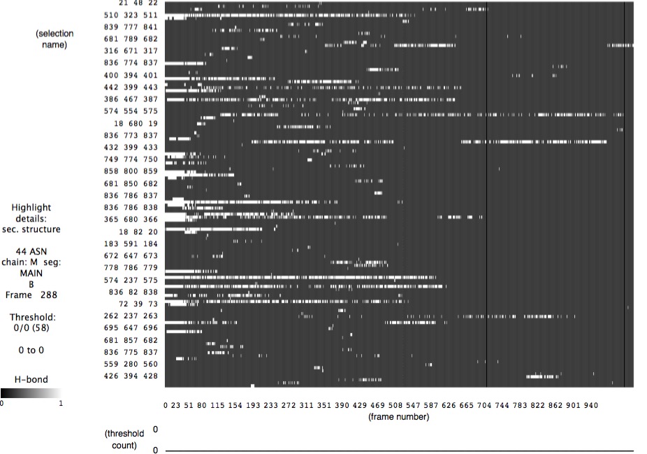
It is useful to use VMD's timeline feature to identify individual hydrogen bonds, and when they break. Recall that this tool shows hydrogen bond triples (atom IDs) versus time. The challenging part is equating this atom ID data with specific locations in the molecule. Many of these "hydrogen bonds" are not really hydrogen bonds by definition. For research purposes, some culling and averaging of data would be necessary.
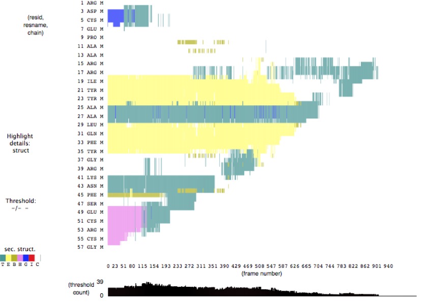
Another way to correlate different data measurements is through VMD Timeline's Secondary Structure feature. This is an example of the secondary structure for the 1qlq molecule from the SMD simulation. Notice how the secondary structural features disappear as the molecule is pulled. Which feature (alpha helix, 3-10 helix, or beta sheet) is the most fragile? Which is the most robust? Together with the Hydrogen Bond feature, you should be able to identify no more than 10 important hydrogen bonds.
tip: you should only have to change names and such for the vacuum simulation. Remember that you have to set up each individual directory for the multiple equilibration steps.
Other Examples
If you would like to try a simpler molecule than 1QLQ, here are two more examples, with suggested pull axes.
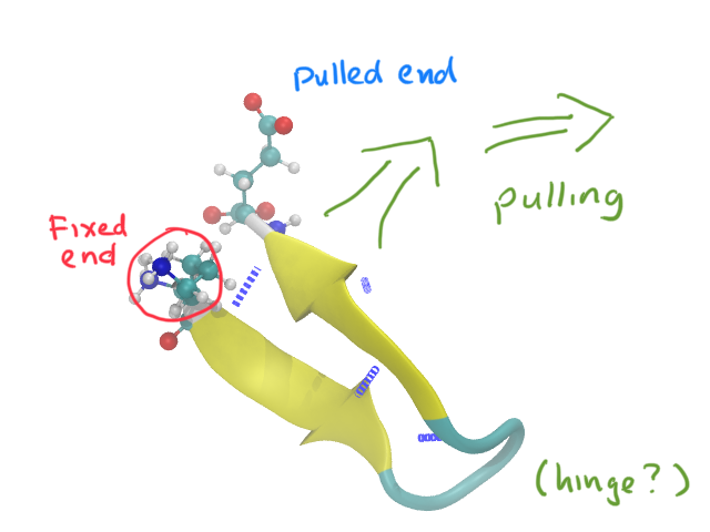
2EVQ is the simplest type of hairpin, a single beta sheet form.
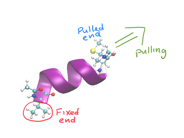
res616 (download link) is a 9 residue fragment of a larger peptide, and provides a nice model for a spring-like system.