There are many useful tools in VMD which allow us to extract useful information. Aside from the very basic tools (picking and measuring tools, for example), there are also a large number of plugins and scripts. Plugins are menu items that researchers have added into VMD in order to extend the basic functionality. A list of such plugins may be found here. Many plugins find their way into the default VMD distribution eventually. We will focus on the “Analysis” type of plugins during this session.
Plugins are usually script files, written in TCL or python (programming languages). In order to uses plugins, you normally have to use the tkconsole, load the file, and then issue commands to extract the functionality. A list of these scripts may be found here. It is relatively simply to learn a bit of TCL or python programming in order to script some repetative task that you might have to do in VMD.
Goals
Explore the basic tools of VMD, including some plugins, and learn basic scripting syntax in order to extend the functionality of VMD.
VMD tools
Mostly found under the “Mouse” main menu item.
query
The query command gives information about the atom clicked on. To enter query mode, type “0” (that’s a zero) in the display window, or select “Mouse...Query” from the main VMD menu. If you click on an atom, and it appears nothing happens, don’t worry. The information shows up in the terminal window that VMD produces when you start the program. An example of the information given:
Info) picked atom:
Info) ------------
Info) molecule id: 2
Info) trajectory frame: 0
Info) name: O
Info) type: O
Info) index: 453
Info) resname: HOH
Info) resid: 74
Info) chain: X
Info) segname: 1PGB
Info) x: 23.827999
Info) y: 9.848000
Info) z: 18.410000
label
The label commands can be activated by selecting “Mouse...Label...”, or by typing 1, 2, 3, or 4 (for atom, bond, angle or dihedral) in the viewer window when it is active. At first glance, label seems to be like query, except it puts a label on the display. However, label includes structural information such as bond length and angular information. Actually, “bond length” really means “distance between two atoms” as the atoms do not need to be bonded. (You will see later that VMD doesn’t really know if atoms are bonded unless we give it addtional information, anyway).
Aside from displaying actual labels on the screen, it makes a list of the labels under the “Graphics...Labels” menu, which pops up a floating window. This is important to remember when you have cluttered your display with many labels, lines and angle markers and you need to get rid of them all.
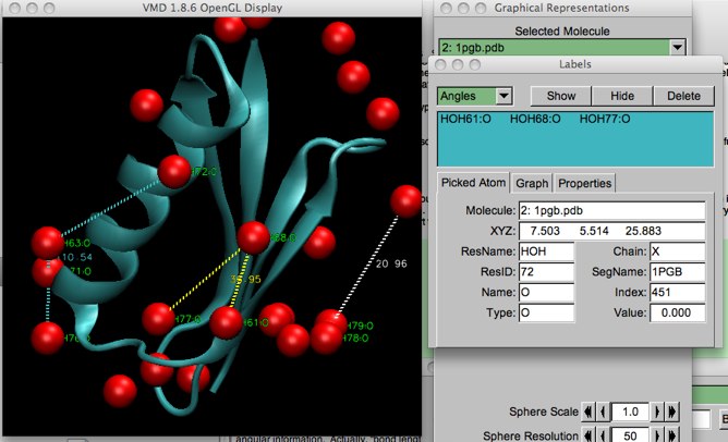
Figure 1: Illustrating the different VMD labels: labels (green); bonds (white); angles (yellow); and dihedrals (blue).
To delete the labels on-screen, simply highlight the label (remember to pull down the proper label type on the left-hand top of the “Labels” menu!), and click “Delete”. You can temporarily hide the label by clicking the “Hide” button.
move
The move command can be activated through the menu as above, or by typing the appropriate number (5, 6, 7, 8) in the main viewer window while it is active. With “move”, you can actually change the coordinates of atoms, fragments, residues, molecules, or representations (recall that each of these definitions are different!). This only changes the coordinates on screen, however, unless you save the new coordinates through the menu or tkconsole.
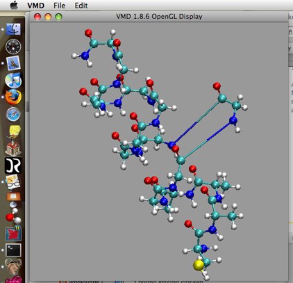
Figure 2: Result of using “move...Residue” (shortcut 6).
So, what if you want to save these changed coordinates? At this point, the easiest thing to do is choose the “File...Save Coordinates” main menu selection. This will cause a save dialog to pop up. You must make sure you choose “all” in the “Selected Atoms” pull-down, and “PDB” in the “File type:” pull down. After you click “Save”, you are prompted for a directory and file name.
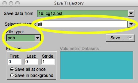
Figure 3: Save coordinates dialog.
Be careful! The VMD User’s Guide has this warning:
Note that there is currently no way to undo Move operations, so the atom coordinates should first be saved to a file.
move lights
With this selection, under “Mouse...Move Light”, you can reposition the virtual lights which illuminate your render. The default set is pretty good, but this can be fun to play with.
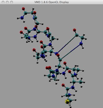
Figure 4: Light 0 has been moved behind the molecule!
Plugins
We will investigate a few plugins now, and use many more of them later on.
RMSD (Extensions..Analysis..RMSD Calculator)
RMSD stands for root-mean-squared deviation. It actually refers to the RMSD of the positions. In order to calculate an RMSD, two (or more) structures must be compared, and one is referred to as the reference structure. The lower the RMSD (usually expressed in angstroms), the more alike the two structures are. RMSD below 2.00 A is generally considered an excellent fit or match. All or part of a protein structure (for example) may be compared. There are further two types of RMSD that are commonly calculated from simulation trajectories: static and dynamic. Static is a one-to-one comparison. Dynamic compares each configuration from a long molecular dynamics trajectory, perhaps 1,000,000 configurations, with a reference structure, usually from NMR or other experimental means.
For now, we will introduce RMSDs with the static, one-to-one structural comparison.
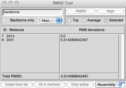
Figure 5: The static RMSD calculator.
Download the two structures 2d1s and 2d1t into VMD. Make sure that you select “New Molecule” for each one or the second won’t load properly. This is a firefly luciferase, responsible for the luminescence of that bug. Once you load these two protein structures, you will see that the total number of atoms differ. If you think about it, this will be a problem since the RMSD compares structures atom-by-atom, and if the structures differ, even by one atom, the math won’t work out!
Open the RMSD tool if you haven’t already. Make sure it is the one labled “RMSD Calculator” not “RMSD Trajectory Tool” (we will use the latter one later on). There may or may not be molecules already loaded in the window. Clear whatever molecules are there by using the “Erase from list” button. Make sure both 2d1s and 2d1t are active, whether or not you have other molecules in VMD; if you do have other molecules loaded, inactivate them. Now, if you click on “Only Active” 2d1s and 2d1t will be loaded into the tool.
On the upper left of the tool is the selection filter. As long as the “Selected” radio button on the right hand side is active, any normal VMD selection will work and filter the molecules. “backbone” is a useful first guess --- it selects the CA (alpha carbons), C (carbonyl carbons) and N (nitrogen) which make up the backbone of every protein. You could also put “all” in the entry box and check the “Backbone only” button, which does the same thing (it is actually like adding “and backbone” to your typed selection). Now hit “Align” (which aligns the molecules using a least-squares algorithm; you may see one of your molecules move during this step), and then “RMSD”. The result is posted below.
What about “Top” and “Average”? Top calculates the RMS distance between the top molecule (which is usually the last molecule loaded) and every other molecule. Average computes the average x, y, z coordinates of the selected atoms in each molecule, then computes the RMS distance of each molecule from that average structure. Thus, if you have a number of molecules loaded, and they either share a backbone, or you can select parts of each you’d like to compare, Top is very useful.
Sequence Viewer (Extensions..Analysis..Sequence Viewer)
The sequence viewer has many functions. Assuming that you have a protein or two loaded into VMD (using the 2d1x proteins above is fine), open up the sequence viewer and let’s have a look. Notice first off the “Molecule” selector. You can switch this between any molecules (molid) you have loaded.
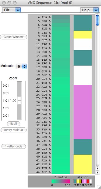
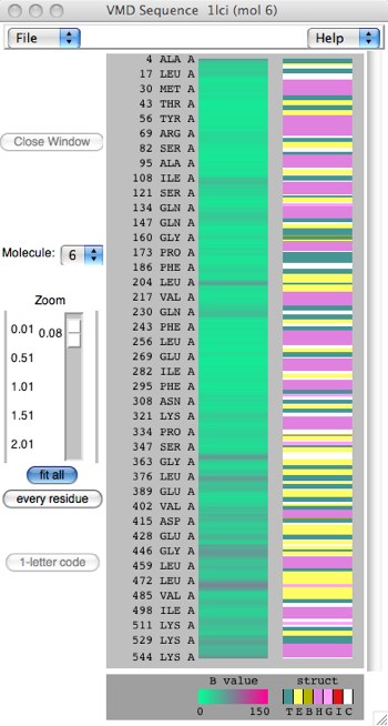
Figure 6: Two different scalings of the Sequence Viewer.
On the left, notice that every residue/amino acid is shown explicitly. Since this sequence is over 500 residues, the view must scroll. This is the result of the “every residue” button. On the right, “fit all” has been clicked, which compacts the sequence to fit the window, losing detail but perhaps showing patterning more clearly. The third colorful column represents the secondary structure of the protein through color-coding (also 1-letter codes as seen under the column): yellow(E) = beta sheet, magenta(H)=alpha helix, cyan(T)=generic turn, white(C)=”no structure”. Other colors are possible: pink(G)=3-10 helix, red(I)=pi helix. You can also toggle between 1-letter and 3-letter amino acid codes.
Go back to your viewer and represent the protein with the “new cartoon” Drawing method and the “structure” Coloring method with a single molecule (turn off the others). The colors should closely match what you see in the sequence viewer. If nothing seems to happen to your viewed molecule, remember that the molecule you want must now be chosen (using the molid pull-down) in three places: the main VMD window, the Graphical Representation window, and the Sequence Viewer window.
(Actually, there is a problem here. The color for the alpha-helix and 3-10 helix are uncomfortably similar in the Sequence Viewer. What color is the 3-10 helix in the “structure” coloring method (you may want to use the select tab to find all 3_10 helix selections...). In fact, the color of the 3-10 helix in the “structure” coloring method was recently changed to better differentiate the two helices. The Sequence Viewer (and the Timeline plugin) have not caught up yet.)
What about that middle column? That is the “B value” field. It turns out that every PDB file has a column set aside for any sort of data a researcher wants to put in. Historically, this is called the temperature column. Later on, we will see how to use this column to make complex decisions with scripting. In this case, we would have to further investigate to understand what these researchers used that column of data to express.
The Sequence viewer has much more to offer. It turns out that you can make selections of your molecule in the Sequence Viewer window! Selections made this way create a new representation with thick yellow bonds. Selections can be made a number of ways: clicking a single residue in the viewer; shift-clicking to add new residues to a previous selection; dragging a rectangle over a series of residues; shift-click and dragging to add new residues to a selection, and right-clicking to deselect.
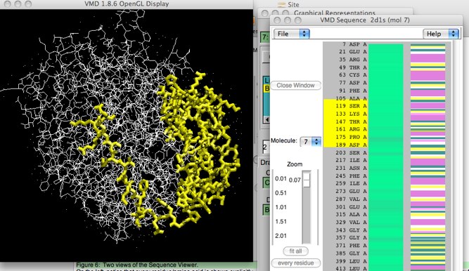
Figure 7: Using the Sequence Viewer to select.
This actually works both ways; if you use the mouse to select an atom/residue/segment in the main viewing window, the selection will show up highlighted in yellow in the sequence viewer, too.
Scripting
Scripting is a little different than using a menu-driven plugin. At first it is harder to enter the commands in a terminal window. Before too long, you realize the flexibility of scripting as you can modify what you have just done easily, and even save your scripting to a file to run it whenever you wish. For now, we will stick to simple scripting in order to get used to the tkconsole. Some basics can be found here.
tkconsole
To begin with, open a tkconsole. This is simply a terminal window using a TCL Shell in which you issue commands (followed by a ) to the program directly. Extensions...Tkconsole will open up the window.
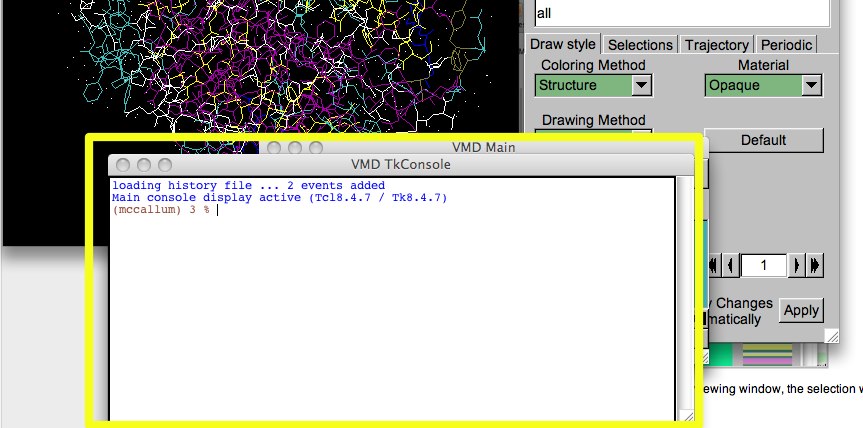 Figure 8: The tkconsole.
One of the nice features of the shell (the program that allows you to send commands to the computer by entering text and hitting “”) is the editability (is that a word?). You can use the up-arrow key on your keyboard to recall earlier commands. You can use the left and right arrows to move through the text and add or delete text. You can delete text by using -d. -a takes you to the beginning of the line, and -e takes you to the end. The tkcon also keeps a history of what you have entered, session-to-session.
Start off by making sure your shell is sitting in the directory where your files are (it is probably in your home directory by default). Type 'pwd'. This will show you which directory you are in. Use 'cd' to appropriately change directories. For example, if I had the directory tree CHEM181/Projects/Project02, I might see this:
[Landau:~] mccallum% pwd
/Users/mccallum
[Landau:~] mccallum% ls -F
CHEM181/ Music/ contactform.html
Desktop/ Network Trash Folder/ dot-tcshrc
Documents/ Pictures/ dot-vmdrc
Downloads/ Public/ etc.hosts
Dropbox/ Res/ scripts/
FileSalvage.dmg Sites/ ss.eps
Google Drive/ SubPC-Cl-NBOm.g03 tcshrc
Home Apps/ auto/ vmd/
Library/ bin/ vmdmovie.tcl
Movies/ colorpts.awk
[Landau:~] mccallum% cd CHEM181/Projects/Project02/
[Landau:~/CHEM181/Projects/Project02] mccallum% ls
project_notes.txt
Once we have the directory properly set, start by deleting all the molecule(s) you may have loaded: typing ‘mol delete all’ at the prompt will do that (don’t forget to hit afterwards!). The viewer should now be empty, and the main VMD window should be blank. Now load a structure that you know from the Protein Data bank by typing ‘mol pdbload 2d1r’ (for example) at the prompt. If you want to load a file from the current directory there is the similar command ‘mol load pdb FILENAME’. Remember that you can follow any output from VMD in the terminal window we saw earlier.
This example protein (2d1r - luciferase) structure has some pesky crystal waters (water molecules that were frozen into the protein structure and showed up in the NMR results), as well as possibly other species such as salt ions and the ligand. Using the graphical representation menu, we can hide these, but using the tkcon we can delete them entirely and save a new pdb of 2d1r without these interlopers. This is very useful! For example, if we would like to run a simulation of the native protein, we must somehow remove the ligand. Also, the crystalline waters might be alright with respect to their positions, but the name ‘HOH” is not typical (as we shall see).
The main command to use is the ‘set VARNAME’ coupled with the ‘atomselect...’ command. ‘set ..’ assigns a set of commands to a variable name. The ‘atomselect....’ command corresponds to making selections (like we did in the ‘Graphical Representations’ window. The general process is:
- select the species
- assign variable names to those selections
- perform an operation on the variable name (the selection)
Here are some example commands. Comments are anything after a ‘#’ symbol --- any text after a hash symbol (#) will be ignored by the tkconsole. This is a handy way to write notes to yourself so you can remember what you were doing when you examine the commands later on.
set all [atomselect top all] # this sets the variable ‘$all’ to include all the atoms in the molecule
set wat [atomselect top "resname HOH"] # “HOH” is the residue name for waters in this file.
set ligand [atomselect top "resname CSO"] # this is the ligand
set protein [atomselect top "not resname HOH and not resname CSO"]
So far, all I have done is set some variable assignments. This is similar to differentiating these residues/species by drawing in the Graphical Representations menu, in a way. To see this, let’s assign some graphical representations using the tkcon rather than the menu. These selections can then be saved to their own PDB files, which now count as independed VMD molecules.
$wat writepdb water.pdb
$ligand writepdb ligand.pdb
$protein writepdb protein.pdb
Now, reload each of the separate PDB files. We have effectively decoupled they from each other. Ensure you can rotate and move them independently.
In general, when we prepare for simulations, each main species type will get it’s own separate PDB. The simulation expects a single PDB for the entire mixture in the simulation box, with some sort of separate label for each specie. In Week 2, we shall see how to do this.
Extracting a single molecule
Now suppose that we would like to make the ligand molecule --- S-hydroxycysteine --- the subject of its own simulation. We have a single CSO molecule, but notice that it is not centered in our viewing area (or in (x,y,z)-space) --- it was bound to a certain part of the luciferase, so we shouldn’t expect it to be centered at (0,0,0). In general, however, it is expected that the PDB of a single molecule is centered at (0,0,0). Let’s see how to do this. We must move the CSO along a vector from the center-of-mass of the molecule to the origin.
Delete all the molecules, and load only the ligand. Notice it doesn’t seem to be offset from the origin. VMD will always center the view of a single molecule on that molecule’s center (of mass). To see this, examine the PDB of the ligand using ‘more ligand.pdb’. A floating window pops up with the coordinates. Hopefully you can see that these are not centered on the origin.
We will use the ‘moveby’ command along with the ‘vecscale’ command (we could also use ‘vecinvert’). Be careful! These commands can be very picky about spaces, etc.
mol delete all
mol load pdb ligand.pdb
set sel [atomselect top all]
set com [measure center $sel weight [$sel get mass]] # output: -4.95155668259 3.86433839798 14.0275144577, which is the center-of-mass
$sel moveby [vecscale -1.0 $com] # also $sel moveby [vecinvert $com]
display resetview
display update ui
$sel writepdb ligand-zeroed.pdb
It is always a good idea to reset the view, and the user interface to make sure you have done what you expect you have done. To convince yourself that our new ligand PDB is actually centered compared to the original, load both PDBs. This new PDB is ready to be used alone, or more likely replicated for use in a simulation.
A common task --- aligning two molecules
Suppose that you have two molecules that are similar, or two different structures extracted from different points in a simulation. You can align these molecules and show how well they match through color coding. As we have seen, the alignment procedure is possible using the RMSD tool, however having the additional way to view the results using color is more interesting.
Load the two small peptide molecules ‘peptideA.pdb’ and ‘peptideB.pdb’ from File Set 1. The following steps will do a best-fit alignment. You will need to use the correct molids for each peptide --- remember you can find these in the Main VMD window after you have loaded them. Here I will assume that the molids are ‘0’ and ‘1’, respectively. The ‘new cartoon’ representation is a good one for this exercise.
mol delete all
mol load pdb peptideA.pdb
mol load pdb peptideB.pdb
set peptideA [atomselect 0 all]
set peptideB [atomselect 1 all]
set M [measure fit $peptideA $peptideB] #this calculates the best-fit matrix “M” - there is some output
$peptideA move $M #peptideA should move to roughly align with peptideB.
Using a supplied script --- coloring.tcl
Here is an example of using a script that someone else has generously supplied (taken from this VMD tutorial). Download the file coloring.tcl, and save it into your current directory. This script will color our two molecules according to how well they align. What it actually does is to add the RMSD value for each atom of the second molecule to the B/beta column of the PDB of the first.. We then manually change the graphical representation to look at that column for color. Simply ‘source’ the file (this reads it), then set the coloring method to ‘beta’.
source coloring.tcl
The color scale range should be set. Find this under “Graphical Representations...Trajectory”. The original scale was 0.46 to 2.17. Change it to 0.0 to 5.0. This changes the molecule to shades of red. To bring back the blue (“good” or low RMSD) to red (“bad” or relatively high RSMD), open up “Graphics...Colors” from the VMD main menu, and select the “Color Scale” tab. The BWR scale means “blue white red”. The “Midpoint” sets what values are white. Since RMSDs must be greater than zero, try setting this around 0.1 or 0.2. The “Offset” can also be adjusted in order to effectively increase the contrast between the two colors.
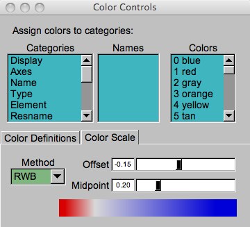
Figure 9: The Color Controls window.
Other useful packages
Orient
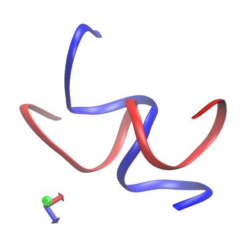
The orient package allows you to align your molecule(s) along one of the principle coordinate axes. Recall that you can turn the axes on or off using the “Display..Axes..” menu item. (Putting the axes at the origin is best if you are going to try and move molecules around.) The orient package is described HERE; you can also download the files at that link, however it may be easier to grab the files orient.tcl and la101.tcl, and put them into the proper VMD directory (VMD.../vmd/scripts/tcl). Once you do this, you need to restart VMD.
Here is an example, using peptideA.pdb (output suppressed):
>Main< (Orient) 91 % package require Orient
>Main< (Orient) 91 % namespace import Orient::orient
>Main< (Orient) 91 % mol load pdb peptideA.pdb
>Main< (Orient) 91 % set sel [atomselect top "all"]
>Main< (Orient) 91 % set I [draw principalaxes $sel]
>Main< (Orient) 91 % set A [orient $sel [lindex $I 2] {0 0 1}]
>Main< (Orient) 91 % $sel move $A
If you do install the Orient package, the documentation tells you to put certain lines in your startup .vmdrc file. For reasons that won't be very clear to you at this point, these instructions are wrong. here are the lines you should put in your .vmdrc file:
catch {lappend auto_path {/Users/chem181/vmd/scripts/extensions/la1.0}};
catch {lappend auto_path {/Users/chem181/vmd/scripts/extensions/orient}};
catch {package require Orient};
catch {namespace import Orient::orient};
Here is the before and after:
Advanced TCL
You may accomplish most of what you can do in the VMD menus through tcl commands in the tkcon. Why would you want to do this? Speed and using scripts (small program files) are the main reason. If you know the commands to use, you can add representations, properly color them, and so on much faster than diving through menus.
>Main< (Hairpin) 75 % mol addrep 0
>Main< (Hairpin) 76 % mol modstyle 1 0 cpk
>Main< (Hairpin) 77 % mol modcolor 1 0 name
This adds a new representation to the molecule with ID 0 (the first rep is number 0, so the first added is number 1); changes the style of that rep to "CPK", and changes the coloring to "name". New representations take on the default values (which can also be modified).
Coloring/Drawing method keywords:
- Secondary Structure: "structure"
- CPK: "cpk"
- HBonds: "hbonds"
You may be able to find out exactly how to modify your representations by using "mol list all":
Status of molecule 2EVQ.pdb:
2EVQ.pdb Atoms:197 Frames (C): 43(42) Status:ADfT
Atom representations: 3
0: on, 197 atoms selected.
Coloring method: structure
Representation: newcartoon
Selection: all
1: on, 197 atoms selected.
Coloring method: ColorID 1
Representation: HBonds 3.000000 20.000000 2.000000
Selection: all
2: on, 109 atoms selected.
Coloring method: Name
Representation: Licorice 0.100000 10.000000 25.000000
Selection: same resname as (index 62 124 70 167 27 174 114 65 118 69 105 74 24 170 31 72 27 177)
From this, you can see how you might for example change the thickness of your licorice representation:
mol modstyle 2 0 licorice 0.4 10 25
Would bring the thickness back to the default of 0.4