In this exercise you will use the supplied trajectories to perform different types of analysis. Many, many more are available --- any type of analyis imaginable. However the most sophisicated analyses usually require running the datasets through various other simulation software, software written by other researchers, or hand-coded programs. We will focus here on analyses avaliable through VMD.
FileSet3.tar.gz
FileSet3.zip
Examples of measurables
Example 1: Energy and other thermodynamic measurables
The energy of the system is an obvious thing to check on, though the actual values themselves are not as interesting as the overall behavior. In other words, it is important that the energy fluctuates, and eventually reaches some sort of general minimum (if an equilibrium system is desired). If there is upward or downward drift, it is a sign that either the system is not equilibrated or there is some sort of “leak” in the energy of the system.
Since the energy calculation in a simulation is made up of many separate parts (van der Waals, electrostatic, dihedral, regular angular, etc), each of these energies may be examined individually also. You may find that some of these energies reach equilibrium more quickly than others. In addition, thermodynamic variables such as temperature, pressure (in constant volume simulations), volume (in constant pressure simulations) and heat capacity may be found rather easily.
How? By default, NAMD prints out a log file to standard output (the terminal). However, if we don’t capture this output in some way, it will scroll off the screen. The solution is to use a redirect symbol to dump this information into a log file:
namd2 alanin.nam > alanin.log
When this job finishes, and control is returned (the cursor comes back), you can view the log file. If you’d like to keep control of your terminal, you can hit -Z to suspend the job, then enter ‘bg’ (which means run the job in the background). If you know you want to run your job in the background to begin with, you can add an amperstand to the end of the command:
namd2 alanin.nam > alanin.log &
If you are wondering how many background jobs you have running in your shell (terminal), you can enter the command ‘jobs’.
Now that we have the log file which contains all the energy information, you can plot it with your favorite plotting program. Since we are not going into depth with such programs here, we will turn to the VMD extension “NAMD Plot” (documentation here):
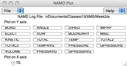
With this extension, you use the “File” menu to load your log file, then choose the variable you’d like to plot (Usually “TOTAL” or “TEMP” (thermodynamic temperature)). To plot the data, choose “Plot data” under the file menu (they really should have used a button for this!). Try this out with your alanin log file.
Example 2: Dynamic RMSD (comparison with experimental structure)
Very often we will want to compare the configurations from our simulations with experimentally-determined structures. An example of this is comparing dynamically-averaged structures determined by NMR to the dynamic simulations. In this case we might load the NMR data as PDBs (single or multiple frames) into one molecule, and loading our simulation data into another. Then we could use the RMSD tool that we saw before to compare the structures. The NMR data would probably be the “Top” molecule (remember if we use the “Top” radio button the top molecule is the reference.
Here is an example. RCSB code 1sse is a reaction center of a YAP1 (Saccharomyces cerevisiae) protein. It consists of 20 frames recorded from NMR experiment. This structure provides a couple different ways to perform RMSDs. First, the 20 configurations can be compared with themselves (or the last 19 can be compared to the first). Open up “Extensions..Analysis..RMSD Trajectory Tool”. Select “Trajectory Frame” to be 0, click “Time” and “Plot”, then click the “RMSD” button.
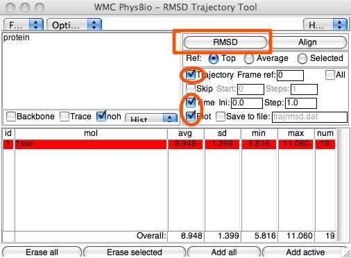
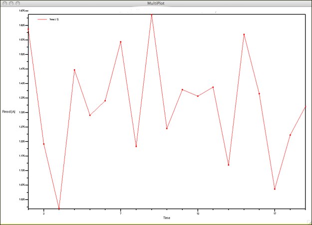
This will give a frame-by-frame RMSD, using the first frame as the reference. The numbers will be rather high, and all over the place. If you study the configurations in the viewer window, however, you might feel this is not in line with what you see. This is because the four main helices are rather static, while the connective peptides are quite mobile. See if you can find a way to bring the for the helices down to what you might expect. (Hint: what can you use in the Graphical Representations window to help with selections? Or in the Sequence Viewer extension?)
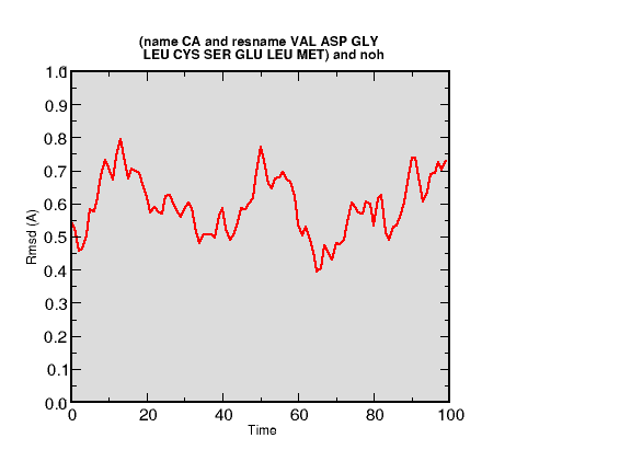
Another way to make this sort of comparison is with a simulation. The files res616.psf, res616.pdb and res616.dcd contain data from a simulation on the helix encompassing residues 598-607 of 1sse. In order to compare this trajectory with one of the NMR structures, we must isolate the part of the 1sse structure that contains this helix. First off, all but one of the 20 frames from 1sse is eliminated. Then, the residues contained in the helix starting at residue number 616 (616 - 624) are selected, and their coordinates written out as a PDB file. Finally, the proper residues are selected in the RMSD Trajectory Tool with the res616 (simulation trajectory) and newly-written 1sse-616 pdb selected. The necessary commands in tkcon are below.
mol load psf res616.psf dcd res616.psf
mol pdbload 1sse
set ref [atomselect top "chain B and resid 616 617 618 619 620 621 622 623 624"]
atomselect16
$ref writepdb 1sse-616.pdb
more 1sse-616.pdb
mol load pdb 1sse-616.pdb
Here is my result (this was plotted in a real plotting program so that you could see the RMSD values clearly). Clearly, this simulated helix closely models the experimental 1sse structure. You can see what selection I used in the RMSD Trajectory Tool in the top of the plot. For a more complete analysis, all 20 1sse configurations would be compared with the trajectory in this manner.
Example 3: Diffusion
Example 4: pair-correlation functions
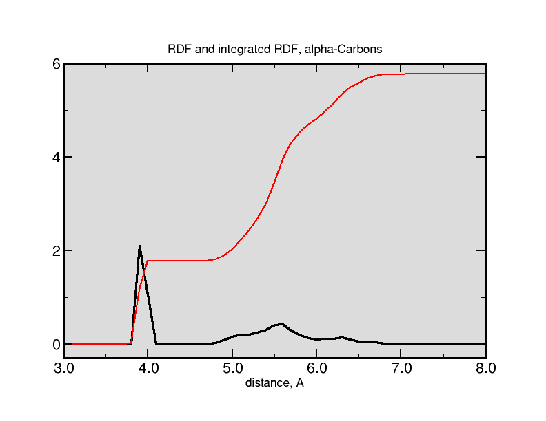
Pair-correlation functions (PCF) are used to show average distances between atoms. Imagine a perfect, hexagonal crystal. There are regular periodic neighbors to some central atom. The probability of finding neighbors is a regular function of distance. You could reconstruct the lattice from the PCF (these functions are sometimes expressed as g(r)). The more certain the positions, the sharper the peaks.
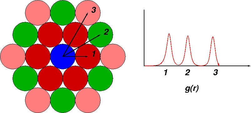
Liquid phases are less organized, but more interesting. These systems are dynamic, of course, so PCFs are very useful when used to describe local interactions. How close are water molecules to the surface of a protein? How are sodium ions arranged around POPE head groups? How many solvation shells of water are gathered around a choride ion?
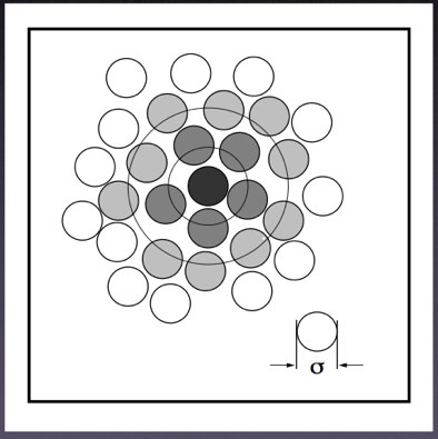
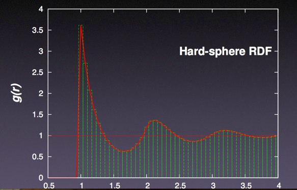
VMD has a very nice extension which allows us to calculate PCFs easily. Load a molecular trajectory and open up the PCF tool (“Extensions...Analysis..Radial Pair Distribution Function”). While PCFs (or RDFs) work best with many free molecules (such as solvent --- water --- or solvated ions), you can still calculate a PCF from a single molecule. Statistics get better with more molecules and more simulation time, so don’t be suprised if your initial functions look noisy or rough.
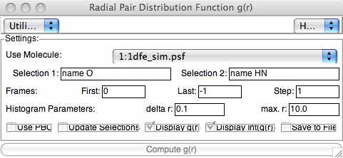
The tool works in the usual way: make two selections for the PCF. For example, if you want to calculate the PCF/RDF for alpha-carbon atoms, both selection 1 and selection 2 would be “name CA”. If you wanted to calculate a PCF/RDF for water-sulfate distances in a simulation beginning from the micelle structure we saw earlier in the class, you might select “name O and resname TIP3” and “name SG” for your two selections. The “Last: -1” Frames selector means “last”; you should not have to fiddle with the Histogram Parameters. If your trajectory data was from a periodically-replicated (periodic boundary conditions) simulation, you would check that box. You can also plot the integrated g(r) --- this gives the total number of neighbors versus distance.
The butane simulation data we examined in week two is a good system to use to explore PCFs.
Here is an example of a CA-CA (alpha carbon) pair correlation function from a trajectory (again from a real plotting program):
Example 5: Hydrogen bonds
Hydrogen bonds are of course very important in most aqueous systems. In proteins they are essentially responsible for protein folding and secondary structure. Hydrogen bonds may be defined in a number of different ways: backbone dihedral angles, O-H-N bond angles, distances, energies, or some combination. Because of this, the exact specification of hydrogen bonds must be spelled out as clearly as possible. Qualitatively, VMD allows the display of hydrogen bonds through the adjustment of geometrical scoring. Quantitatively, hydrogen bond analysis requires re-running trajectories through analysis programs, usually hand-written by research groups.
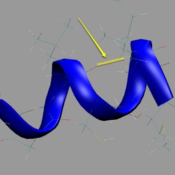
We will use VMD in order to qualitatively understand hydrogen bonding. Load a peptide trajectory (ek or ck or res598 or res616). Create a representation for the peptide or protein, and create a new representation which uses “Color ID” for coloring and “HBonds” for Drawing method. It is best to pick a bright color for Color ID, and adjust the line thickness or else you might not see the hydrogen bonds. Remember that each representation can have it’s own smoothing window under the “Trajectory” tab.
There is also a hydrogen-bond analysis tool with the Timeline (Calculate -> Calc. HBonds). When called, a window pops up which lets you define the angle and distance parameters. After that, the hydrogen bond occupancy is calculated, and something like this appears:
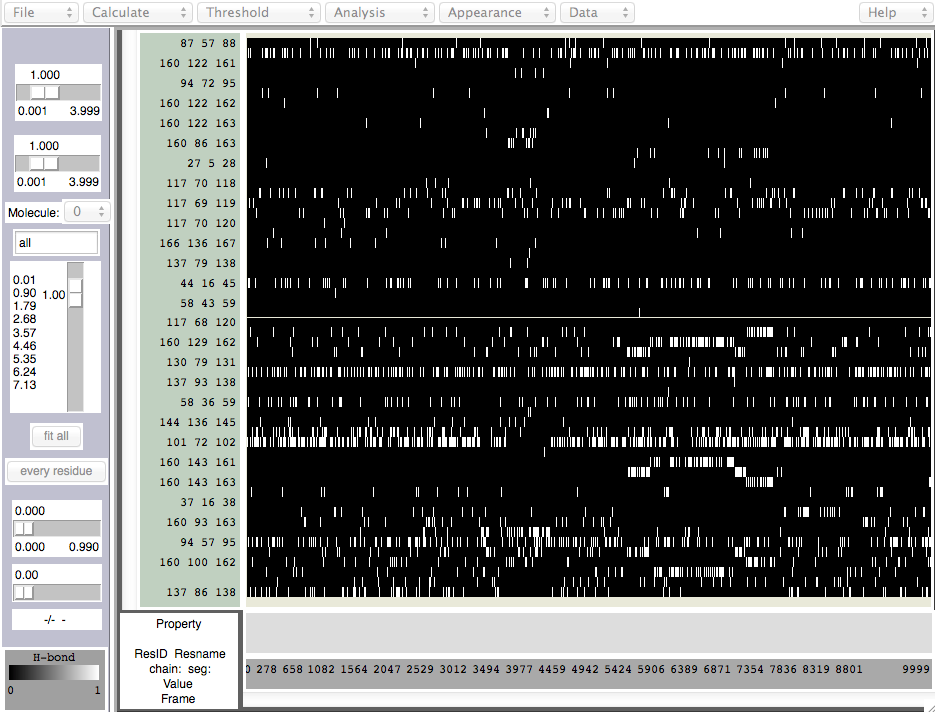
White shows the hydrogen bond is "on", and black is "off". Many of these are not alpha-helical hydrogen bonds, and most are transient and/or unimportant. Further analysis can be done by using the "File.." menu to write the data.
There is yet another HBond analysis tool: VMD: "Analysis -> Hydrogen Bond":
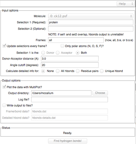
A lot of information can be obtained here if you ask to "Calculate detailed info for: All hbonds". If you do so, make sure you write out the data to a file so you can use a real plotting program.
Some questions to think about when investigating hydrogen bonds are:
- At what locations do hydrogen bonds occur?
- What is the lifetime of an average hydrogen bond?
- How many hydrogen bonds occur at the same time, on average?
- How does solvent affect the above?