Trajectories are files that contain coordinates for all the atoms over the course of the simulation. Usually, not every finite time step of the simulation is saved: every 100 or 500 or 1000 steps saved is common. What exactly is a step? Well, Molecular Dynamics integrates Newton’s equations, using the forces applied on each atom from its neighbors to move it around. In order to do this, time is broken up into discrete timesteps, usually 1 or 2 fs (1 fs = 10-15 sec). Thus, in order to get a (barely) meaningful simulation experiment of 10 ns, one would need 10 million timesteps of 1fs each.
Each trajectory file is essentially a PDB file for each saved timestep. The common format we will use (from CHARMM and/or NAMD) is a .dcd file. These are usually binary (machine-readable), not ASCII (human-readable), as binary files are much smaller than ASCII, and all those coordinates add up! Having all these coordinates means that we are able to measure dynamic properties of our simulation experments: secondary-structure evolution, diffusion constants, correlations between groups, and so on. This gives us a powerful quantitative tool.
In addition, we can make movies using this data. This will be covered in the next topic.
For this exercise, we will use three sets of data: Two (similar) peptides and a collection of butane molecules (You can get the files individually: ek12.psf ek12.dcd ck12.psf ck12.dcd butane.psf butane.pdb butane.dcd butane.trj or everything as a .tar.gz archive: FileSet2).
Loading Trajectories
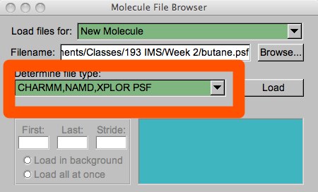
In order to load a trajectory, we need both the PSF and the trajectory file. As usual, you can load this through the menu or through the tkcon. In the menu, the PSF should always be loaded first. Very often, the file auto-detect in VMD gets the file type wrong, so you should always check to make sure this is set to the correct filetype.
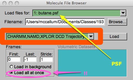
Once you have the ‘butane.psf’ PSF loaded (don’t forget to hit “Load”), you can browse to the DCD file. You should notice you are loading files for the ‘butane.psf’ (yellow arrow in picture below). Browse to the ‘butane.dcd’ file. In this case, you must make sure the filetype is set to “CHARMM,NAMD,XPLOR DCD...” (orange). Even if the suffix of your file was something strange like “.trj” or “.lop”, if you set this properly, the file will be read properly. It is also a good idea to click the “Load all at once” button (magenta) or else you will have to wait while VMD moves through the DCD file frame-by-frame. I don’t know why this isn’t the default behavior...
When you are done, you should see a roughly cubical box of butanes. Go ahead and represent them however you want.
Skipping/eliminating frames
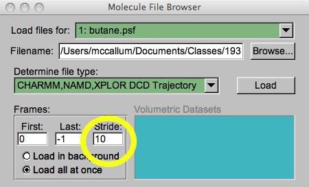
Sometimes these DCD files will be large, and you only want an idea of what the data looks like. Or, the simulation may have saved data every 10 timesteps, and you want to cut it down to every 100 or 500 timesteps. In these cases, you may want to skip some regular number of frames. This is easy to do while loading. You can set the first frame to load, the last frame to load, and the “Stride”, which tells you the skipping step. In the example below, I am going to load every 10th frame of the whole trajectory.
Viewing the trajectory
Now you can view the trajectory, movie-like, by clicking on the play button (see below). You will probably have to adjust the speed of the playback: experiment with the “Loop” pulldown and the “step” and “speed” controls. The “step” command allows you to skip frames in playback. The difference (from the loading step) is that these frames are still there, they are simply not viewed. So any analysis, statistics, etc. will still include them.
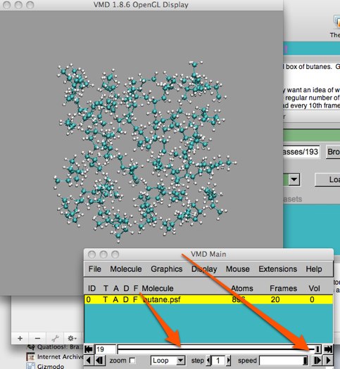
Notice how jumpy this “movie” looks with the step set to 1. Changing this step doesn’t seem to help the jerkyness much, does it?
Smoothing (versus eliminating frames)
The real answer to making the movie look smoother is found under the Graphical Representations menu. Open that menu up, and click on the “Trajectory” tab. You will find a “Trajectory Smoothing Window Size” control. This allows interpolation of the moves, averaged over the number you set here. I have found “5” works pretty well. Once this is set, you should find you are able to follow individual butane molecules around the box. You may notice some molecules disappearing from one side, and reappearing on the other. This is due to periodic boundary conditions. Simply put, periodic boundary conditions (PBC) tries to simulate many more molecules than you are actually using by replicating the simulation box with periodic images in all directions. In two dimensions, this is like putting your simulation box at the center of a checkerboard, and making copies of that box to fill the other checkerboard squares. Thus, when a molecule leaves the box in one direction, it re-enters the box on the opposite side.
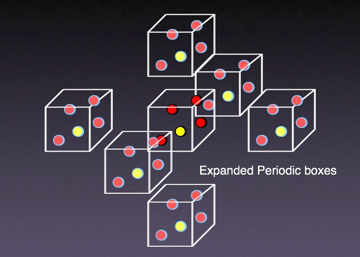
VMD can account for this by displaying periodic images, something we will work with later on.
Simple dynamic analysis via labels
The simplest way to begin to use VMD to analyze trajectories is through labels. We saw labels earlier, but now they become more useful. Let’s start with something simple. Load the PSF/DCD pair for ck12 (from FileSet2). This trajectory has 10,000 frames, which is probably too much at first glance. Let’s cut it down to 1,000. This can be done by selecting a stride of 10 when loading, or by using the “Delete Frames” menu selection (From “File...Delete Frames” or by right-clicking on the molecule name in the list, in the main VMD window), and choosing a stride of 10.
To begin, let’s measure the end-to-end distance over time. This will have something to do with the helical nature of this peptide, as a nicely-formed helix will be longer than a random coil. For picking out individual atoms, CPK is probably the best representation. Set your cursor on Label/bond mode (or type “2” with the focus on the viewer window), and choose two atoms on each end of the molecule. Now if you run the trajectory, this distance will adjust as the atoms move about. It may help you visualize the molecule if you add a representation and make it “ribbons” or “new cartoon”. If you are going to use Trajectory smoothing (see above), each representation can have it’s own smoothing window size.
This end-to-end length information is nice to see on screen, but what if we would like to plot the data separately? Open up the “Graphics...labels” form. Pull down “bonds”, and click on the “Graph” tab. If you now click on “Show Preview”, a mini-plot will show up. The minimum and maximum values are labeled along with the trajectory frame number.
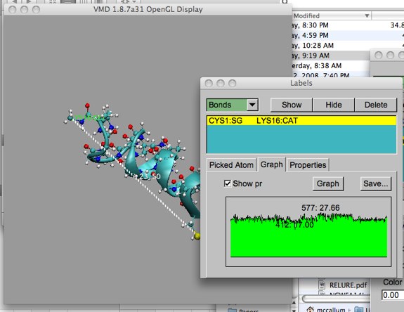
You have two other options here. First, you can pop up another, larger graph window by clicking the “Graph” button (orange, below). You can also save the data to a file by clicking the “Save..” button (blue arrow below). Though we won’t discuss plotting data in great detail in this course, this is a valuable resource to have for publishing results.
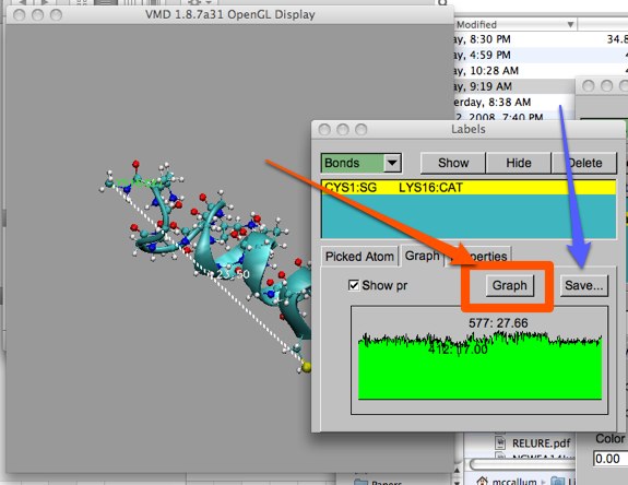
Any other sort of information that can be labeled may be plotted in this way.
Dynamic RMSD
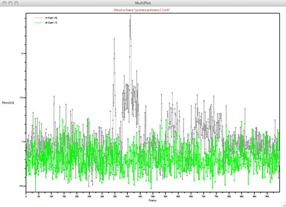
Earlier we used RMSDs to compare structural details. Time-evolution of structural details can be followed by using dynamic RMSD. Here we will compare two similar peptides, ek12 and ck12. The only difference is that ck12 has an N-terminal cysteine in place of an alanine in ek12. Load both PSF/PDB pairs into VMD, and once again load only 1,000 frames.
Opening up “Extensions...Analysis..RMSD Trajectory Tool” (description here) will open up a window somewhat similar to our earlier RMSD tool. Since the two molecules have the same number of residues, if we choose “protein” or “backbone” we should be able to get an alignment without any errors. Notice that there are several new choices here, related to the trajectory. These should be straightforward to figure out with our experience. The reference can be once again “Top”, “Average” or “Selected” (use “Average” for this example). The choices below are related to trajectories. The reference frame can be set, along with a skip (stride) interval. If “All” is selected, each frame from the top molecule is compared with each frame in the other molecule(s) --- this takes much longer! The time can also be set (for plotting); these times are in femtoseconds. Finally, the results can be plotted and/or sent to a file.
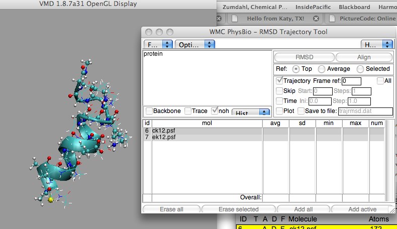
Here is a typical result:
Trajectory coloring by structure
One of the nicer features in VMD is the ability to draw in secondary structure and label the structure by color, using a combination of ‘cartoon’ or ‘new cartoon’ and coloring by ‘structure’. Load either ek12 or ck12, and set up this representation combination. As you watch the trajectory unfold, you may be thinking how static the alpha-helix form is in this molecule. The trouble is, VMD is giving the wrong impression. It turns out that the coloring and structural representation for the whole trajectory is set by the structure of the first frame! How can we get VMD to re-calculate the color and structure frame-by-frame?
You may think that if you click ‘Trajectory...update color every frame’ under the Graphical Representations menu, the color (at least) will change, but this turns out not to be so for this coloring representation. Fortunately, there is a script called ‘sscache.tcl’ which will accomplish this for us. Here is the documentation. Save this file somewhere convenient, and source it in your tkcon: ‘source sscache.tcl’. Once the file is sourced, you may run the commands contained in the file.
In order to have sscache color your molecule trajectory, you must start and stop it. The commands are:
start_sscache molid - start caching the given molecule
stop_sscache molid - stop caching
reset_sscache - reset the cache
A word about using the tkcon: This is actually a "terminal" or shell, a very common (and somewhat old-fashioned) way to send commands. The short snippet of text before the cursor is the prompt. The prompt is often used to show status. In the tkcon, the prompt will show you your current working directory (the folder that you are "sitting in"; this is analogous to opening that folder in OS X Finder or Windows). Another nice thing about the shells we will be using is command completion. The shell allows you to complete command names and/or file names by using the key.
Using the above example of sourcing the sscache.tcl file, and assuming the file is in your current working
Start the sscache for your molecule (remember to enter the molid). Now if you reset your trajectory back to the beginning, and run it again, you will notice both the structural (cartoon) and color changing over time (it will probably appear to flicker back and forth between colors and ribbon width). The first time through the trajectory, it will run noticeably more slowly as the information is cached. Succeeding times will run much more quickly.
How can we make a movie!? We will do that in the next exercise.
DSS plots
DSS stands for ‘determination of secondary structure’. Presta and Rose devised this way to describe secondary structure; in fact it is the way the coloring by structure is done in VMD. Another way to visualize such information is through a DSS timeline. This is similar to a movie spread out in a 2D plot.
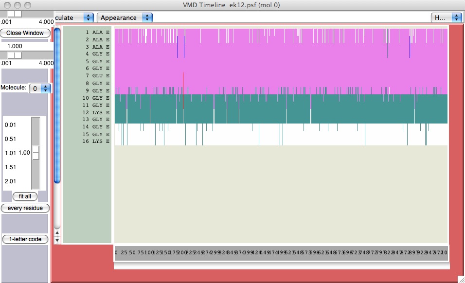
From the Extensions menu, choose “Analysis..Timeline”. When you first open it up, the trajectory will run. Pull down “Calculate Secondary Structure”. The trajectory will run again, and presently a color plot will come up. The y-axis represents the residues (primary structure), and the x-axis is simulation timesteps. See how this compares with the representation of the trajectory you showed, above.
